Analyzing Hydrologic Time-Series for Flood Frequency Analysis
This content delves into the methods and assumptions involved in studying hydrologic time-series data for flood frequency analysis. It covers topics such as different types of assumptions, including independence and persistence, and highlights how streamflow data can be analyzed to find annual maximum values. The material also discusses the insights that can be gained from studying time-series data, such as extracting information, making assumptions, estimating values or probabilities, and the types of analysis required for each aspect.

Analyzing Hydrologic Time-Series for Flood Frequency Analysis
PowerPoint presentation about 'Analyzing Hydrologic Time-Series for Flood Frequency Analysis'. This presentation describes the topic on This content delves into the methods and assumptions involved in studying hydrologic time-series data for flood frequency analysis. It covers topics such as different types of assumptions, including independence and persistence, and highlights how streamflow data can be analyzed to find annual maximum values. The material also discusses the insights that can be gained from studying time-series data, such as extracting information, making assumptions, estimating values or probabilities, and the types of analysis required for each aspect.. Download this presentation absolutely free.
Presentation Transcript
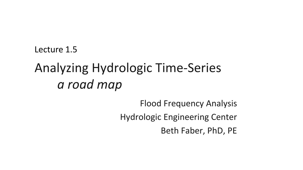
Lecture 1.5 Analyzing Hydrologic Time-Series a road map Flood Frequency Analysis Hydrologic Engineering Center Beth Faber, PhD, PE
Goals Review (or preview) some ways we might study a time-series, and what we can learn from it 1. What information we extract 2. What assumptions we make 3. What values or probabilities we can estimate 4. What type of analysis each requires 2
Assumption Assumption Topics independence independence Annual Extremes annual maximums or minimums, Bulletin 17B/C instantaneous flows or longer duration avg flow/volume independence independence Partial Duration (peaks over threshold) Daily flows or stages Duration Curves Summary Hydrographs Annual Volumes Drought, Dependent random variables No independence No independence - - persistence persistence No independence No independence - - persistence persistence 3 3
Assumption Assumption Topics independence independence Annual Extremes annual maximums or minimums, Bulletin 17B/C instantaneous flows or longer duration avg flow/volume independence independence Partial Duration (peaks over threshold) Daily flows or stages Duration Curves Summary Hydrographs Annual Volumes Drought, Dependent random variables No independence No independence - - persistence persistence No independence No independence - - persistence persistence 4 4
Streamflow data, daily flow record American River at Fair Oakes (unregulated) American River at Fair Oaks (unregulated) 300000 108 years of daily unregulated streamflow data 250000 average daily flow (cfs) 200000 150000 100000 50000 0 Nov-04 Oct-14 Oct-24 Oct-34 Oct-44 Oct-54 Oct-64 Oct-74 Oct-84 Oct-94 Oct-04 reservoir constructed 5
Streamflow data, find annual max American River at Fair Oakes (unregulated) American River at Fair Oaks (unregulated) 300000 consider each year's maximum flow 250000 often, annual peaks are often, annual peaks are instantaneous instantaneous values values average daily flow (cfs) 200000 150000 100000 50000 0 Nov-04 Oct-14 Oct-24 Oct-34 Oct-44 Oct-54 Oct-64 Oct-74 Oct-84 Oct-94 Oct-04 6
American River, ANNUAL MAX SERIES, AMS annual maximum values are independent annual maximum values are independent 300000 108 years of annual peak flow data 250000 Annual Peak Streamflow (cfs) 200000 150000 100000 50000 0 1926 1931 1935 1939 1944 1948 1974 1978 1983 1987 1991 1905 1909 1913 1918 1922 1952 1957 1961 1965 1970 1996 2000 2004 2009 7 7
Assumptions What we have: series of annual maximum flows Treat these flows as a random, representative sample from the population of interest -- -- probability distribution of annual probability distribution of annual peak flow peak flow Generally, we assume the sample is IID annual peak flows are random and independent peak flows are identically distributed homogeneous data set sample is adequately representative of the population (but estimate of the distribution improves with sample size) NOTE, since we collect data over time, we re assuming the data/watershed is stationary . 8
Histogram divide data range into bins, count number of observations in each bin (frequency), divide by total (relative frequency) 0.45 0.41 0.4 0.33 0.35 0.3 relative frequency 0.25 0.2 count/obs 0.13 0.15 0.1 0.04 0.04 0.010.030.020.00 0.000.01 0.05 0 37.5 62.5 87.5 112.5137.5162.5187.5212.5237.5262.5 0 25 50 75 100 125 150 175 200 225 250 275 Flow, in thousands of CFS this shape is similar to a PDF, probability density function this shape is similar to a PDF, probability density function 9 9
Histogram divide data range into bins, count number of observations in each bin (frequency), divide by total (relative frequency) 0.25 0.21 0.2 0.18 0.18 switch switch to to log log10 (flow) 0.15 relative frequency 0.13 0.11 10(flow) 0.1 count/obs 0.07 0.06 0.04 0.05 0.02 0.010.00 0.01 0 3.4 3.6 3.8 3.2 3.4 3.6 3.8 4.0 4.2 4.4 4.6 4.8 5.0 5.2 5.4 5.6 4 4.2 4.4 4.6 4.8 5 5.2 5.4 5.6 Log (Flow, in thousands of CFS) Log Flow (thousands of CFS) this shape is similar to a PDF, probability density function this shape is similar to a PDF, probability density function 10 10
Definition of PDF and CDF 0.2 A Probability Density Function (PDF), f(x), defines the probability of occurrence for a continuous random variable. area under curve = probability area under curve = probability PDF Probability per Unit Value 0.15 0.1 p 0.05 0 X of Variable X Value The Cumulative Distribution Function (CDF), F(x) is the probability the random variable is less than some value curve = probability curve = probability 1 0.8 Probability Less Than CDF 0.6 0.4 0.2 p 11 0 11 X of Variable X Value
Empirical Cumulative Distribution based on observation based on observation Empirical or Graphical estimate: based on order statistics, using plotting position (estimated non-exceedance probability) Cumulative probability of observation magnitude is based on its position within the sample, and the sample size Each observation has incremental prob = 1/N mi relative relative frequency frequency i.e., i.e., N mi = rank of ordered observation i (m=1 as smallest value, N as largest) N = total # of observations P[X xi] = estimate probability that outcome will be smaller than observation x estimate probability that outcome will be smaller than observation xi i by the fraction of the observed sample that by the fraction of the observed sample that is is smaller than x smaller than xi i 12 12
Plotting Positions Want to avoid a value equal to 1 (N/N)! Some common plotting positions: m Weibull N + 1 p = mean estimate of probability p =m 0.3 Median N + 0.4 median estimate of probability Hirsch-Stedinger based on threshold-exceedance where m = rank N = total # of values
Empirical Cumulative Distribution plotting position plotting position Non-Excdnc Probability Non-Excdnc Probability Year Rank Flow Year Rank Flow Plotting Position: 1997 108 252431 0.99 1955 14 10528 0.13 1955 107 189073 0.98 1975 13 10389 0.12 1964 106 183242 0.97 1972 12 10046 0.11 General Formula P =m + a 1986 105 170960 0.96 2008 11 9150 0.10 2005 104 161731 0.95 1966 10 8659 0.09 1963 103 152614 0.94 1939 9 8500 0.08 1950 102 132000 0.94 1907 8 8460 0.07 N + b 1980 101 124915 0.93 2001 7 8045 0.06 1928 100 119000 0.92 1931 6 7920 0.06 Weibull: a = 0.0, b = 1.0 Median: a = -0.3, b = 0.4 1982 99 113126 0.91 1990 5 7606 0.05 1907 98 105000 0.90 1961 4 6914 0.04 1909 97 98000 0.89 1988 3 5447 0.03 1970 96 88316 0.88 1994 2 5009 0.02 1969 95 83526 0.87 1977 1 2359 0.01 14
Empirical Cumulative Distribution Exceedance Probability Estimated from Plotting Positions 1.00 cumulative non-exceedance probability 0.90 0.80 0.70 CDF = cumulative CDF = cumulative distribution function distribution function 0.60 0.50 0.40 0.30 0.20 0.10 0.00 0 50000 100000 150000 200000 250000 300000 Annual Peak Flow (cfs) 15 15
Empirical Cumulative Distribution Exceedance Probability Estimated from Plotting Positions 300000 for a Corps for a Corps frequency curve, frequency curve, we switch axes... we switch axes... 250000 annual peak flow (cfs) 200000 150000 100000 50000 0 0.00 0.10 0.20 0.30 0.40 0.50 0.60 0.70 0.80 0.90 1.00 cumulative non-exceedance probability 16 16 annual
Empirical Cumulative Distribution also called a frequency curve also called a frequency curve Exceedance Probability Estimated from Plotting Positions 300000 250000 ...and adjust axis scales ...and adjust axis scales annual peak flow (cfs) 200000 150000 100000 50000 Normal probability scale Normal probability scale 0 0 0.01 0.05 0.1 0.2 0.5 0.8 0.9 0.95 0.99 1 cumulative non-exceedance probability 17 17 annual
Empirical Cumulative Distribution also called a frequency curve also called a frequency curve Exceedance Probability Estimated from Plotting Positions 1000000 log log scale scale ...and adjust axis scales ...and adjust axis scales annual peak flow (cfs) 100000 10000 Normal probability scale Normal probability scale 1000 0 0.01 0.05 0.1 0.2 0.5 0.8 0.9 0.95 0.99 1 cumulative non-exceedance probability 18 18 annual
Empirical Cumulative Distribution also called a frequency curve also called a frequency curve Exceedance Probability Estimated from Plotting Positions 1.01 Return Period 5 100 2 20 10 1000000 log log scale scale largest in 108 years, probability 1/108 0.9% equaled or exceeded 11 times in 108 years 10% switch to switch to exceedance exceedance annual peak flow (cfs) 100000 Weibull would Weibull would be 1/109 be 1/109 10000 0.9% Normal probability scale Normal probability scale 1000 1 0.99 0.95 0.9 0.8 0.5 0.2 0.1 0.05 0.01 0 cumulative exceedance probability Cumulative Exceedance Probability 19 19 Annual
Empirical Graphical Cumulative Distribution Exceedance Probability Estimated from Plotting Positions 1.01 Return Period 5 100 2 20 10 1000000 log log scale scale annual peak flow (cfs) 100000 10000 Normal probability scale Normal probability scale 1000 1 0.99 0.95 0.9 0.8 0.5 0.2 0.1 0.05 0.01 0 cumulative exceedance probability Cumulative Exceedance Probability 20 20 Annual
for unregulated, for unregulated, instantaneous annual instantaneous annual maximums maximums Analytical Distribution Exceedance Probability Estimated from Plotting Positions 1.01 Return Period 5 100 2 20 10 1000000 log log scale scale Log Pearson III per Bulletin 17B/C annual peak flow (cfs) 100000 10000 Normal probability scale Normal probability scale 1000 1 0.99 0.95 0.9 0.8 0.5 0.2 0.1 0.05 0.01 0 cumulative exceedance probability Cumulative Exceedance Probability 21 21 Annual
Distribution Fitting a model for probability: Step 1: Choose Model Step 2: Calibrate Model (Estimate Distribution Parameters) Can estimate population parameters using sample statistics. The general descriptive parameters are: Distribution Moments Central Tendencywhere? Dispersion or Spreadhow wide? where? (location) (location) how wide? (scale) (scale) (shape) (shape) Asymmetry symmetrical? symmetrical? PDF 22
Sample Standard Deviation Sample Skew Coefficient Sample Mean N N N Xi X3 N X =1 1 Xi X2 N i=1 Xi S = N 1 g = i=1 (N 1)(N 2) S3 i=1 average distance average distance from mean from mean where: Xi = sample member, i N = sample size dimensionless dimensionless g g = 0 has same unit has same unit as variable as variable g g < 0 S g g > 0 23
Distribution Moments First moment: mean X = N i=1 1 NXi Second central moment: variance Sx Xi X2 1 N 2= N 1 i=1 Third standardized central moment: skew gx= N 1 N 2 Sx N 1 N Xi X3 3 i=1 24
Distribution Parameters CDF, frequency curve form CDF, frequency curve form 1400000 1200000 1000000 Streamflow (cfs) Peak difference in difference in the mean the mean 800000 600000 400000 difference in the difference in the standard deviation standard deviation 200000 0 99 95 90 75 50 25 10 5 1 0.1 Exceedence Frequency 100 x probability of exceeding 100 x probability of exceeding 25
Distribution Parameters CDF, frequency curve form CDF, frequency curve form 1400000 1200000 1000000 Streamflow (cfs) Peak negative negative skew = 0 is skew = 0 is straight line straight line on this on this Normal prob Normal prob axis axis 800000 changing changing the skew the skew 600000 400000 positive positive 200000 0 99 95 90 75 50 25 10 5 1 0.1 Exceedence Frequency 100 x probability of exceeding 100 x probability of exceeding 26
for unregulated, for unregulated, instantaneous annual instantaneous annual maximums maximums Analytical Distribution Exceedance Probability Estimated from Plotting Positions 1.01 Return Period 5 100 2 20 10 1000000 log log scale scale Log Pearson III per Bulletin 17B/C annual peak flow (cfs) 100000 10000 Normal probability scale Normal probability scale 1000 1 0.99 0.95 0.9 0.8 0.5 0.2 0.1 0.05 0.01 0 cumulative exceedance probability Cumulative Exceedance Probability 27 27 Annual
Bulletin 17B dated March 1982 Bulletin 17C dated Feb 2018 28 28
B17B/C: Frequency Analysis of Annual Peak Flows Estimate LogPearson III distribution for unregulated annual peak flows Method of Moments moments of sample used to estimate moments of distribution Data challenges: Missing Flows (Broken or Incomplete Record) Low and High Outliers Zero Flows Additional information to improve estimates: Historical/Paleo Information Regional Skews (use a weighted skew) Allowing a longer record site to improve short record estimate many of the methods many of the methods for handling data for handling data challenges and using challenges and using additional information additional information are improved in are improved in Bulletin 17C Bulletin 17C 29 29
for unregulated, for unregulated, instantaneous annual instantaneous annual maximums maximums Analytical Distribution Exceedance Probability Estimated from Plotting Positions 1.01 Return Period 5 100 2 20 10 1000000 log log scale scale Log Pearson III per Bulletin 17B/C annual peak flow (cfs) 100000 90% confidence interval 10000 Normal probability scale Normal probability scale 1000 1 0.99 0.95 0.9 0.8 0.5 0.2 0.1 0.05 0.01 0 cumulative exceedance probability Cumulative Exceedance Probability 30 30 Annual
Also Interested in Regulated Flow Reservoir Storage Level Inflow 160,000 cfs 115,000 cfs Release 31 31
Streamflow data, regulated American River below Folsom Reservoir 300000 period of record 1955 - 2009 homogeneous homogeneous = = identically identically- - distributed distributed = = stationary stationary 250000 Is this regulation homogeneous? Is this regulation homogeneous? average daily flow (cfs) 200000 150000 100000 50000 0 Nov-04 Oct-14 Oct-24 Oct-34 Oct-44 Oct-54 Oct-64 Oct-74 Oct-84 Oct-94 Oct-04 reservoir constructed 32 32
Streamflow data, regulated American River below Folsom Reservoir 300000 period of record 1921 - 2002 250000 2 benefits: 2 benefits: these are simulated outflows: these are simulated outflows: average daily flow (cfs) 200000 homogeneous homogeneous operation, operation, and longer and longer period period HOMOGENEOUS operation HOMOGENEOUS operation 150000 100000 50000 0 Nov-04 Oct-14 Oct-24 Oct-34 Oct-44 Oct-54 Oct-64 Oct-74 Oct-84 Oct-94 Oct-04 33 33
Streamflow data, regulated American River below Folsom Reservoir 300000 consider each year's maximum flow 250000 regulated annual peaks regulated annual peaks average daily flow (cfs) 200000 150000 100000 50000 0 Nov-04 Oct-14 Oct-24 Oct-34 Oct-44 Oct-54 Oct-64 Oct-74 Oct-84 Oct-94 Oct-04 34 34
Folsom Release, ANNUAL MAX annual maximum values are independent annual maximum values are independent 300000 300000 108 years of annual peak flow data 81 years of annual peak flow data 250000 250000 Annual Peak Streamflow (cfs) Annual Peak Streamflow (cfs) 200000 200000 150000 150000 100000 100000 50000 50000 0 0 1926 1931 1935 1939 1944 1948 1974 1978 1983 1987 1991 1905 1909 1913 1918 1922 1926 1931 1935 1939 1944 1948 1952 1957 1961 1965 1970 1974 1978 1983 1987 1991 1996 2000 2004 2009 1905 1909 1913 1918 1922 1952 1957 1961 1965 1970 1996 2000 2004 2009 35 35
Plotted Annual Maximums Exceedance Probability Estimated from Plotting Positions 1.01 Return Period 5 100 2 20 10 1000000 annual peak flow (cfs) 100000 10000 1000 1 0.99 0.95 0.9 0.8 0.5 0.2 0.1 0.05 0.01 0 cumulative exceedance probability Cumulative Exceedance Probability 36 36
Does an Analytical Curve Make Sense? Exceedance Probability Estimated from Plotting Positions 1.01 Return Period 5 100 2 20 10 1000000 annual peak flow (cfs) 100000 10000 1000 1 0.99 0.95 0.9 0.8 0.5 0.2 0.1 0.05 0.01 0 cumulative exceedance probability Cumulative Exceedance Probability 37 37
Graphical Curve is Better for this Exceedance Probability Estimated from Plotting Positions 1.01 Return Period 5 100 2 20 10 1000000 annual peak flow (cfs) 100000 10000 1000 1 0.99 0.95 0.9 0.8 0.5 0.2 0.1 0.05 0.01 0 cumulative exceedance probability Cumulative Exceedance Probability 38 38
Graphical Curve is Better for this Exceedance Probability Estimated from Plotting Positions 1.01 Return Period 5 100 2 20 10 1000000 annual peak flow (cfs) 100000 how do we how do we extrapolate? extrapolate? 10000 1000 0.99 0.95 0.9 0.8 0.5 0.2 0.1 0.05 0.01 cumulative exceedance probability Cumulative Exceedance Probability 39 39
Extending a Regulated Curve To extend a regulated frequency curve, we can construct synthetic events with a specified frequency, e.g. 100-yr, 200-yr, etc Estimate frequency curves for longer duration average flows or volumes (3-day, 7-day, 30-day, etc) Construct hydrograph for a given frequency Route through operation model to get peak outflow NOTE: will assume likelihood of peak release is related to likelihood of peak inflow 4040
Graphical Curve is Better for this Exceedance Probability Estimated from Plotting Positions 1.01 Return Period 5 100 2 20 10 200 500 1000000 annual peak flow (cfs) 100000 10000 1000 0.99 0.95 0.9 0.8 0.5 0.2 0.1 0.05 0.01 cumulative exceedance probability Cumulative Exceedance Probability 41 41
Assumption Assumption Topics independence independence Annual Extremes annual maximums or minimums, Bulletin 17B/C Instantaneous flows or longer duration avg flow/volume independence independence Partial Duration (peaks over threshold) Daily flows or stages Duration Curves Summary Hydrographs Annual Volumes Drought, Dependent random variables No independence No independence - - persistence persistence No independence No independence - - persistence persistence 42 42
Longer Durations of Flow/Volume Volume Frequency Analysis Create a family of frequency curves for a given site that specify average flow across various durations 1. Compute m-day moving average TS for various durations, m m might be 1-day, 5-day, 30-day etc. 2. Extract annual maximums for each duration 3. Perform frequency analysis for each duration Similar to Bulletin 17B/C procedure, but not instantaneous peak Compute plotting positions and distribution parameters from each period of record sample 43 43
Longer Durations Max Average Flows 1-day AMS 1-day Daily Average 5-day AMS 5-day Daily Average 10-day AMS 10-day Daily Average 44 44
Longer Duration Max Average Flows 120000 Kootenai River @ Libby daily 1day Unregulated Streamflow (cfs) 100000 15day 30day 80000 60day 90day 60000 40000 20000 0 1-Feb-70 2-Aug-70 31-Jan-71 1-Aug-71 30-Jan-72 30-Jul-72 28-Jan-73 29-Jul-73 27-Jan-74 28-Jul-74 4545
Max Flow at Folsom Volume-Freq Curves Note: average flow easier to plot than volume curves are closer 1DAY 3DAY 7DAY 15DAY 30DAY shorter duration shorter duration (1 day) is more (1 day) is more extreme extreme Percent Chance Exceedance 47 47
Note: its important to define the year define a year that won t break up longer high flow averages what about for low flows? 48 48
Synthetic Events rare rare Create synthetic, low-frequency event hydrographs to model extremes, or other watershed conditions (e.g. regulated flow) 1. perform volume frequency analysis produce the family of m-day average flow frequency curves 2. choose an historical event as a hydrograph shape 3. scale the hydrograph to match flow of chosen exceedance probabilities (e.g., the 1% chance event) read the average flow for each duration for the chosen exceedance probabilities scale the hydrograph up or down to match that avg flow 49 49
Max Flow at Folsom Volume-Freq Curves 1/200-year 1DAY 3DAY 7DAY 15DAY 30DAY shorter duration shorter duration (1 day) is more (1 day) is more extreme extreme Percent Chance Exceedance 50 50
Rescaling Historical Event 1997 flood event 500000 American River @ Folsom 450000 Unregulated Streamflow (cfs) 400000 350000 1997 hourly 1day 300000 0.6% chance exc 3day 250000 7day 15day 200000 1.0% 0.97% 150000 0.8% 100000 1.2% 50000 0 12/19 12/23 12/27 12/31 1/4 1/8 1/12 1/16 51 51