CERTIFIED BUSINESS MANAGEMENT ANALYST

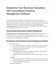
Certified Business Management Analyst specializing in Manufacturing Operations, Retail Management, and Service Management Analysis. Services include cost savings analysis, make-or-buy decisions, production automation alternatives, and break-even analysis. Case studies provided for practical application.

CERTIFIED BUSINESS MANAGEMENT ANALYST
PowerPoint presentation about 'CERTIFIED BUSINESS MANAGEMENT ANALYST'. This presentation describes the topic on Certified Business Management Analyst specializing in Manufacturing Operations, Retail Management, and Service Management Analysis. Services include cost savings analysis, make-or-buy decisions, production automation alternatives, and break-even analysis. Case studies provided for practical application.. Download this presentation absolutely free.
Presentation Transcript
CERTIFIED BUSINESS MANAGEMENT ANALYST 13) Manufacturing Operations Analysis 14) Retail Management Analysis 15) Service Management Analysis
13) Manufacturing Operations Analysis Costs Savings Manufacturing Make-or-Buy Analysis Product Tree Structure Inventory Levels at Work Center Production Job Scheduling Materials Scheduling Work Center Performance Analysis Work Center Load Balancing Analysis Production Automation Alternatives Cycle Counting of Inventories Operations-Lead-Times and Queuing Models Kanban Containers Machine Setup Cost and Time Service Levels and Lead Times Demand During Lead Times Plant Layout Production Cycle Time and Workstations Preventive Maintenance Management 1. 2. 3. 4. 5. 6. 7. 8. 9. 10. 11. 12. 13. 14. 15. 16. 17. 18.
Costs Savings Much expenditure is associated with manufacturing operations (materials, machines, labor, money, energy etc). Cost saving is one of the criteria for initiating automation projects. Consider both fixed costs and variable cost/unit for different production alternatives. The alternative with maximum cost savings should be selected. Manufacturing Make-or-Buy Analysis Decide whether to buy a part or component from outside or to produce the part of component by considering fixed costs and variable costs for all alternatives. The alternative with the least total cost should be selected.
Production Automation Alternatives Break-even analysis can help management in making a chose between a manual & semi-automatic production process for a new product line. Both Fixed costs and variable costs are considered for all alternatives.
Questions 284 & 285, page: 185 In XYZ company, one of the engineers prepared a proposal to change from a job shop to a cellular manufacturing settings. The cost for the current job shop and the proposed cellular setting are summarized in below table, assuming the annual production volume of 100,000 unit: Present job shop Cellular proposal $50,000 $2.5 Annual fixed costs Variable cost/unit $115,000 $1.6 Production volume: 100,000 unit What would be the annual cost savings if this proposal was accepted? At what point volume would this company be indifferent toward the proposal? Present job shop Cellular proposal $300,000.0 $72,222.22 Total cost Break even point $275,000.0
Questions 286-289, page: 186 WXC company wants to decide whether to buy a product it uses or to produce the product itself. It expects to need 50,000 unit per year and has the following three options: Buy Porduct Produce Manually Produce Automated $0 $150,000 $20 $18 Fixed costs Variable costs $200,000 $15 What should the WXC company do regarding this product? At what point volume would this company be indifferent to buying the product or producing it manually? At what point volume would this company be indifferent to buying the product or producing it by automated production? At what point volume would this company be indifferent to buying the product or producing it by automated production? Buy Porduct Produce Manually Produce Automated Total cost $1,000,000 $1,050,000 $950,000 1&2 1&3 2&3 75,000 40,000 16,667
Product Tree Structure Product Tree: a graphical representation of the bill of material (BOM). Used to show the quantities required per each component. BOM: a listing of all of the raw materials, parts, subassemblies, and assemblies needed to produce one unit of a product. RMs Components sub- assemblies Assemblies FG Assume that Product Z is made up of two units of A and four units of B. A is made of three units of C and four units of D. D is made of two units of E. Draw a product tree for Z. A (2) C (3) D (4) E (2) Z B (4)
Product Tree Structure Level 0 Chair Leg Assembly Back Assembly 1 Seat Cross bar Side Rails (2) Cross bar Back Supports (3) Legs (2) 2 3
Inventory Levels at Work Center Most manufacturers divide inventory into: Raw materials (RM) - materials and components scheduled for use in making a product. Work in process - WIP - materials and components that have begun their transformation to finished goods. Finished goods (FG) - goods ready for sale to customers. I. II. III. To calculate inventory level at a work center compare: Actual inputs to planned inputs Actual outputs to planned outputs Calculate Work In Process (WIP)
Production Job Scheduling Which order or job to process first?! How to sequence jobs? Consider average flow time, average flow rate, or total changeover costs etc. Some of the sequencing / dispatching rules: First-come, First-Served (FCFS) Next job to be produced is the one that arrived first among the waiting jobs. Shortest Processing Time (SPT) Next job to be produced is the one with the shortest processing time among the waiting jobs. Critical Ration (CR) Next job to be produced is the one with the least CR time among the waiting jobs. CR = time to promised delivery for a job/production time for that job Least Changeover Cost Select jobs sequence that would minimize total changeover costs.
Average Flow Time & Number of jobs Total waiting time = Summation of waiting time for all jobs. Average waiting time = Total waiting time/number of jobs Average number of jobs in the shop = Total waiting time/total processing time
Questions 294-299, page: 189 A print shop has 4 jobs to be processed through their only five-color press. Production times for each job are as follows: Production time (min) 30 17 12 39 Time to promised delivery (min) 25 22 15 45 Job A B C D At what order should the four jobs be done using the SPT rule? C-B-A-D What is the average waiting (flow) time for all jobs using the SPT? Average waiting time = (12+29+59+98)/4 = = 198/4 = 49.5 min What s the average number of jobs in shop using the SPT rule? Average number of jobs in shop= (12+29+59+98)/98 = 198/98 = 2.02 job What is the average waiting (flow) time for all jobs using the FCFS rule? Average waiting time = (30+47+59+98)/4 = = 234/4 = 58.5 min What s the average number of jobs in shop using the FCFS rule? Average number of jobs in shop= (30+47+59+98)/98 = 234/98 = 2.39 job What s the first job to be processes using the critical ratio rule? CRA = 25/300.83, choose Job A
Materials Scheduling Material requirements planning (MRP): Computer-based information system for ordering and scheduling of dependent demand inventories. Using MRP improves customer service, reduce investment in inventory, and improve operating efficiency of a plant. Dependent demand: Demand for items that are subassemblies or component parts to be used in production of finished goods. Master Production Schedule (MPS): Time-phased plan specifying timing and quantity of production for each end item. Inputs to MRP: Gross requirements for a product (taken from MPS), Scheduled receipts, and beginning inventory.
Work Center Performance Analysis Productive time per hour : The number of minutes in each hour that a workstation is working on the average. A workstation may not be working because of such things as lunch ,personal time , breakdowns, start-ups, and shutdowns. Workstation : Physical location where a particular set of tasks is performed. Workstation are usually of two types : a manned workstation containing one worker who operates machines and/or tools, and an unmanned workstation containing unattended machines. Work center : A physical location where two or more identical workstations are located .If more than one workstation is required to provide enough production capacity ,they are combined to form a work center.
Work Center Performance Analysis How to determine if manufacturing resources are being utilized efficiently and effectively? Utilization % = (Hours Actually Worked / Available Hours)* 100% Efficiency % = (Standard Hours of Work Produced / Hours Actually Worked )* 100% Available Capacity = Available Time in Hours X Utilization% X Efficiency % Measured (demonstrated) capacity is an average of previous production output.
Work Center Performance Analysis A manufacturing plant has a work center that produced 135 standard hours of work over the past week. This work center was available for 160 hrs, and actually worked 120 hrs. Over the previous 4 weeks, the same work center produced 150, 130, 120 and 140 standard hrs of work. What s the utilization %, Efficiently %, available capacity, and measured capacity for this work center? Utilization % = 120/160 * 100% = 75% Efficiency % = 135/120 *100% = 112.5% Available Capacity = 135 hrs Measured (demonstrated) capacity= (150+130+120+140)/4= 135
Work Center Load Balancing Analysis Load : amount of planned work scheduled for and actual work released to a facility, work center, or operation for a specific span of time. Expressed in terms of Standard hours of work of units of production. Load balancing (leveling): spreading work orders out in time or rescheduling operations so that the amount of work make it more economical to produce in larger lots than are needed for immediate purposes. Total load = released load + planned load. Under or over capacity = total load variable capacity Over capacity work center is overloaded Under capacity work center is under-loaded
Production Cycle Time and Workstations Incremental utilization heuristic Minimum number of workstation : The least number of workstation that can provide the required production, calculate by: Theoretical minimum # of workstations = ( task times per unit) * demand (piece/hr) / productive time (min/hr) = Sum of all tasks times/Cycle time Cycle time : The time in minutes between products coming off the end of a production line Cycle time = productive time (min/hr) / demand (piece/hr) Example (Page 204): For XYZ company that s considering improving their lines by using Incremental utilization heuristic, if the productive time/hr = 55 min, the demand is 23 piece/hr, and the tasks details for their assembly line are available in below table, find the following: Task A B C D E F G Predecessor - A A B C D, E F Duration 0.5 3.25 1 2 2.25 1 0.25 1- Cycle time 2- Theoretical minimum # of workstations
Cycle Counting of Inventories A cycle count is an inventory management procedure where a small subset of inventory is counted on any given day. Cycle counts are less disruptive than physical inventory to daily operations, and provide an ongoing measure of inventory accuracy and procedure execution, and can be tailored to focus on items with higher value, higher movement volume, or that are critical to business processes. Most cycle counting applications use an ABC analysis, segregating items into various count frequencies. ABC inventory classification system would help in prioritizing items for cycle counting.
Operations-Lead-Times and Queuing Models Operations-Lead-Times: the period of time between the initiation of any process of production and the completion of that process. Some queue structures: First come first served (FCFS) Last come first served (LCFS) Service in random order Priority service Balance arrival rates with processing rates using Queuing Models.
Kanban Containers Kanban (kahn-bahn) is a Japanese word that when translated literally means visible record or card developed by Toyota, refers to cards used to control the flow of production through a factory. Kanban is a JIT production method. kanbans are signals used to replenish the inventory of items used repetitively within a facility in pull system.. The typical kanban signal is an empty container designed to hold a standard quantity of material or parts. When the container is empty, the customer sends it back to the supplier. The container has attached to it instructions for refilling the container such as the part number, description, quantity, customer, supplier, and purchase or work order number. Steps followed for replenishing stock in Kanban system: A container has just been emptied at the Drilling station. The kanban is placed in the kanban collection box. The full containers at Milling, with kanbans attached to them, are transported to Drilling and the kanbans in the collection box are taken back to Milling. Milling continues to fill containers depending on the demand from Drilling. Empty containers are collected from Drilling periodically. Management is interested in reducing the number of containers and in increasing the efficiency rating.
Machine Setup Cost and Time With each machine setup a cost is associated due to maintenance personnel and materials involved it changeover process. The necessary setup cost is computed as following: EOQ = [(2DS/C)(p/(p-d))]^0.5 S = [C*(EOQ^2)/2D][(p-d)/p] where: D: annual demand, d: daily demand p: daily production rate C: carrying cost per item S: setup cost Setup Time = Setup Cost / Labor Rate
Service Levels and Lead Times Lead time is the period between a customer's order and delivery of the final product. Service level is the probability that a stockout will not occur during LT. Must be > 95% Specify demand during LT to reduce stockouts probability. Assuming demand during LT is normally distributed based on the past date. ROP (Re-Order Point) is determined as follows: ROP/OP = EDDLT + SS Required service level affects Safety Stock (SS). SS = OP EDDLT Where OP : Order Point, also called ROP EDDLT: Expected demand during lead time
Plant Layout Plant Layout: the physical arrangement of everything needed for the product or service, including machines, personnel, raw materials, and finished goods. The criteria for a good layout necessarily relate to people (personnel and customers), materials (raw, finished, and in process), machines, and their interactions. Some of the factors used to determine plant layout: ease of future expansion or change, flow of movement, materials handling, space utilization, ease of communication and support, and safety. Space has to be utilized efficiently by considering expected movement of products between departments & requested area for each department. Departments that have the highest amount of product movement between them should be located close to each other. Departments that have no product between them should be located at opposite ends of the building..
Preventive Maintenance Management Preventive maintenance is a schedule of planned maintenance actions aimed at the prevention of breakdowns and failures / malfunctions. The primary goal of preventive maintenance is to prevent the failure of equipment before it actually occurs. It is designed to preserve and enhance equipment reliability by replacing worn components before they actually fail, or by machine adjustments, lubrications, cleaning, painting, and needed repair and overhaul work. Having standby machines reduces costs associated with breakdown; lost of production time, overtime usage on the other machines, and emergency repair procedures. Nevertheless, having standby machines would result in storage and special handling expenses. The number of standby machines needed is calculated using the expected values and relative probabilities to minimize expected costs. Long-term benefits of preventive maintenance include: Improved system reliability. Decreased cost of replacement. Decreased system downtime. Better spares inventory management.
Preventive Maintenance Management One of the preventive maintenance measures is the repair rate for vehicles ( ). Formula: = + 1/ ts Where: : average or mean service rate : average or mean arrival rate ts: the average waiting time in the system and is computed as 1/( - ) Number of mechanics = /vehicles per mechanic per week : average or mean service rate : average or mean arrival rate
Preventive Maintenance Management BTC Inc. has a fleet of 600 vehicles. Based on historical records, an average of 14 vehicles/week require repair work. These records show that on average, each mechanic can repair four vehicles/week. Company policy requires vehicles to be back in service in 0.5 week on average. The repair rate is number of vehicles repaired be week. What s the average repair rate for vehicles at BTC Inc. Company? ts: 1/( - ) = + 1/ ts = 14 + 1/0.5 = 16 vehicle/week How many repair mechanics are required at the BTC Inc. Company? Number of mechanics = /vehicles per mechanic per week Number of mechanics = 16/4 = 4 mechanics
Preventive Maintenance Management XYZ company has 900 employees, each using a computer terminal. When a terminal stops functioning, if a spare is not immediately available on site, it costs, the company an average of $ 100 in lost employee productivity before a new terminal can be obtained. For each spare terminal that the company keeps on site but does not use, it is estimated that the cost is $25/week for storages, insurance, and opportunity cost. The demand pattern for the terminals is as follows: Weekly Demand 15 20 25 30 Total Relative Frequencies 0.21 0.35 0.30 0.14 1.00 What s the expected cost for keeping twenty terminals in stock? How many terminals should be stocked to minimize expected costs? What s the cost of stocking 20 terminals if 25 are needed? Occurances 22 37 32 15 106 Terminals required/wk Terminals stocked/wk 15 20 25 30 Answers: page 206-207 15 0 500 1000 1500 20 125 0 500 1000 25 250 125 0 500 30 375 250 125 0
14) Retail Management Analysis Merchandize Pricing Merchandise Planning Merchandise Control Retail Inventory Valuation Methods Retail Inventory Pricing Systems Summary of LIFO and FIFO Methods Merchandise Profitability Analysis Retail Inventory Turns and Levels Store Productivity and Performance Net Requirements Schedule Economic Order Quantity and Costs Fixed Order Period Model ABC Inventory Classification System Retail Store Layout 1. 2. 3. 4. 5. 6. 7. 8. 9. 10. 11. 12. 13. 14.
Merchandize Pricing Merchandize pricings decision and retail decisions must be made together. Selling price = Cost/(100%-Markup%) Selling price = Cost + Markup in $ Markup % on cost = (Price-Cost)/Cost Initial Markup% = (Operating Expenses + Profits + Reductions)/(Net sales + Reduction) Maintained Markup% = Initial Markup%-[(Reduction%)*(100%-Initial Markup%) Reduction % = Amount of reduction /Net Sales Maintained Markup is the difference between the actual selling price and the cost of that merchandise, is more important that the initial markup.
Merchandise Planning Methods used for planning dollars invested in merchandise/ merchandise planning systems: The basic stock method BOM stock= (average stock average monthly sale)+ planned monthly sales The percentage variation method BOM stock = average stock for a season * 0.5*[1+(planned sales for the month/average monthly sales)] The week s supply method BOM stock= average weekly sales * the number of weeks to be stocked The stock-to-sales ratio method BOM stock= stock-to-sales ration * planned monthly sales A combination of the preceding four methods % variation, week s supply and stock-to-sales ratio methods are good when the turnover rate is more than 6.
Merchandise Control Merchandise control is critical to ensure an adequate level of stock is on hand for the amount of sales being generated. Having too much inventory (or the wrong type) during certain periods can slow your cash flow and reduce profits with too many markdowns. Markdown: Planned reduction in the selling price of an item, usually to take effect either within a certain number of days after seasonal merchandise is received or at a specific date Open to Buy (OTB) amount: the dollar amount that a buyer can currently spend anytime during the merchandise period without exceeding the planned amount of merchandise. Open to Buy (OTB) method: Method for a retailer to adjust merchandise purchases to reflect changes in sales, markdowns, and so on. The open- to-buy method provides flexibility for the retailer in purchasing new inventory as the old items sell out and to take advantage of special product deals.
Open to Buy (OTB) method The Open-To-Buy Formula Planned Sales + Planned Markdowns + Planned End of Month (EOM) Inventory - Planned Beginning of Month (BOM) Inventory - Commitments at retail for delivery ---------------------------------------- = Open-To-Buy (retail)
Retail Inventory Valuation Methods Methods used for valuating a retailer s inventory: I. Cost Method II. Retail method (most commonly used, oldest and most useful) III. Lower of Cost or Market (LCM) method. Ending book inventory value accuracy depends on free of errors recording for: BOM inventory, purchases, freight-in, markups, markdowns, discounts, returns, transfer between stores, and sales. Formula used in inventory valuation: Cost compliment of book inventory = total cost valuation / total retail valuation. Ending Inventory at cost = adjusted ending book value at retail with the cost complement book inventory. COGS = total inventory valuation at cost ending inventory at cost Gross margin = Sales COGS Net profit before taxes = Gross profit total operating expenses.
Cost of Goods Sold Analysis Cost of Goods Sold Analysis Definition: The direct costs attributable to the production of the goods sold by a company. This amount includes the cost of the materials used in creating the good along with the direct labor costs used to produce the good Equation COGS = RM Used in Production + Manufacturing Expenses + Diff. in Inventory Balances
Retail Inventory Pricing Systems Inventory pricing systems for retailers: First in and first-out (FIFO) Last-in and first-out (LIFO) FIFO and LIFO yield different values for ending inventories and COGS when identical units of a particular product have been acquired at different prices. Each method has advantages and disadvantages LIFO Most preferred to be used for planning because it reflect replacement costs. Cushion the impact of inflationary pressures by matching current costs with current revenues. COGS is based on the costs of items purchased most recently. Older inventory is regarded as unsold inventory FIFO: best represents true merchandise cost, assumes that the oldest merchandise is sold first. Assumes that the older merchandise is sold before the more recently purchased merchandise.
Summary of LIFO and FIFO Methods Pricing System Ending inventory value COGS Gross margin Net income Taxes LIFO Lower Higher Lower Lower Lower FIFO Higher Lower Higher Higher Higher
Merchandise Profitability Analysis Profit/Gross Margin / Net Profit / Net Income / Operating Profit Bottom line: net income after taxes Operating Profit: A measure of a company's earning power from ongoing operations, equal to earnings before deduction of interest payments and income taxes (EBIT). The difference between the Net Profit and the operating profit will be the interest expense and the taxes The following formulas can be used in assessing the profitability of a store or retailer: Annual Sales = total number of transactions * average transaction size Gross Margin = Sales COGS Gross Margin Amount = Gross Margin % * Sales Gross Margin % = Gross Margin / Sales Total Operating Costs = total variable costs + total fixed costs. Operating Profit = Gross Margin - Total Operating Cost Net income after taxes = Operating Profit Interests Taxes Closure rate = total number of transactions/annual store traffic (# of customers)
Retail Inventory Turns and Levels Inventory turnover is the number of times per year, on average, that a retailer sells its inventory. Inventory Turnover Ratio = Annual Sales/Average Inventory at Retail Or = COGS/Average Inventory Retailers are classified into the following groups: Low-margin/low-trunover retailers. Low-margin/high-trunover retailers. High-margin/low-trunover retailers. High-margin/high-trunover retailers. High-performance retailers are those who achieve financial excellence in terms of high gross margin percent, high inventory turnover ratio, and high net income after taxes.
Store Productivity and Performance Productivity = Profit Measuring productivity of a retailer: Space Productivity = net sales / total square feet of retail floor space Labor Productivity = net sales / number of fulltime equivalent employees. Merchandize Productivity = net sales / average dollar investment in inventory= Sales to stock ratio Sales Productivity = net sales / number of customers. i. ii. iii. iv. Return on Asset (ROA): An indicator of how profitable a company is relative to its total assets/ resources. ROA is calculated by dividing a company's annual earnings by its total assets.
Net Requirements Schedule Net Requirements Schedule for a product indicates how many units should be released to purchasing. Can be calculated using the following formula: Net requirements = estimated demand + ending inventory beginning inventory Estimated demand : gross requirements
Economic Order Quantity (EOQ) and Costs EOQ: is the lot sizes that minimize total annual inventory holding and ordering costs to keep inventories low enough to avoid excess inventory holding costs but high enough to reduce ordering and setup costs. We use EOQ If we follow a make to stock strategy and the items has relatively stable demand. If you are carrying costs and setup or ordering costs are known and relatively stable. We don t use the EOQ If you use the make to order strategy and your customer specifies the entire order to be delivered in one shipment. If the order size is constrained by capacity limitation such as number of delivery trucks.
Economic Order Quantity (EOQ) and Costs Calculating EOQ Total stocking cost = Q/2*C + D/Q*S Tom minimize both acquiring and carrying costs, Q becomes: EOQ= (2DS/C) Where Q: average current order quantity C=cost of holding/ carrying one unit in inventory for 1 year D= annual demand in units per year S=cost of ordering or setting up one lot, in dollar per lot.
Fixed Order Period Model Fixed order period = T = (2S/DC) Order Quantity = Upper inventory target Current inventory level + EDDLT Total stocking cost (TSU) = DT/2*C + S/T Where T: Time interval for ordering
ABC Inventory Classification System ABC analysis : an inventory categorization technique used in materials management through identifying items which will have a significant impact on overall inventory cost & providing a mechanism for identifying different categories of stock that will require different management and controls. When carrying out an ABC analysis, inventory items are valued (item cost multiplied by quantity issued/consumed in period) with the results then ranked. The results are then grouped typically into three bands. These bands are called ABC codes: "A class" inventory will typically contain items that account for 50-70% of total value, or 10-20% of total items. "B class" inventory will have around 20% of total value, or 20% of total items. "C class" inventory will account for the remaining 10-30% of total value, or 60-70% of total items.
Retail Store Layout Maximize the following two elements of store layout to maximize sales: Store image: The overall perception the consumer has of the store s environment. I. Space productivity: How effectively the retailer utilized it s space and is usually measured by: Sales/square foot of selling space. Gross margin dollars/square foot of selling space. II. Decision rules for better store layout include the following:. Departments that have the most hourly customer traffic between them should be located next to each other. Departments that have the least hourly customer traffic between them should be located farthest from each other.
15) Service Management Analysis Service Management; introduction Yield Management Forecasting Retail Store Sales Efficient Retail Stores Profitable Sales Call Service Facility Layout Site Location Departmental Work Sequence Waiting Line Management 1. 2. 3. 4. 5. 6. 7. 8. 9.
g o o d s and s e r v i c e s Goods - things you can touch - tangible Services - things you can t touch - but you can see their effect intangible services are not physical, they are intangible
Service A Service is a type of a product. a deed performed by one party for another Services have special characteristics that make them different than products. A product without physical characteristics; a bundle of performance and symbolic attributes designed to produce consumer want satisfaction.
Tangible / Intangible Attributes Tangible touch see taste smell Intangible can t see can t touch can t smell can t taste GOODS SERVICES

 Manufacturing Operations Analysis")


 Retail Management Analysis")


 method")


 and Costs")
 and Costs")


 Service Management Analysis")