Explanation of the infinitesimal dipole element used in wire antennas, calculation of radiated fields, radiation patterns, directivity, and far-field patterns. Includes illustrations and equations for a comprehensive understanding.

• Antenna Patterns
• Infinitesimal Dipole
• Directivity
• Radiation Patterns
• Electromagnetics

nadine Follow

Uploaded on Apr 19, 2024 | 4 Views

Understanding Antenna Patterns and Directivity of Infinitesimal Dipole Elements

PowerPoint presentation about 'Understanding Antenna Patterns and Directivity of Infinitesimal Dipole Elements'. This presentation describes the topic on Explanation of the infinitesimal dipole element used in wire antennas, calculation of radiated fields, radiation patterns, directivity, and far-field patterns. Includes illustrations and equations for a comprehensive understanding.. Download this presentation absolutely free.

Presentation Transcript

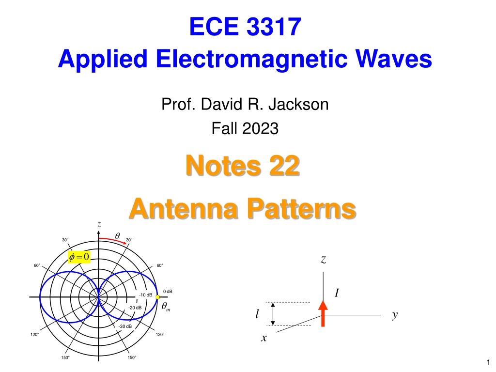
1. ECE 3317 Applied Electromagnetic Waves Prof. David R. Jackson Fall 2023 Notes 22 Antenna Patterns z 30 30 z = 0 60 60 I 0 dB -10 dB -20 dB m l y -30 dB x 120 120 150 150 1

2. Infinitesimal Dipole The infinitesimal dipole current element is shown below. z I l y x The dipole moment (amplitude) is defined as Il. The infinitesimal dipole is the foundation for many practical wire antennas. From Maxwell s equations we can calculate the fields radiated by this source (e.g., see Chapter 14 of the Hayt and Buck textbook). 2

3. Infinitesimal Dipole (cont.) The exact fields of the infinitesimal dipole in spherical coordinates are 1 r 1 Il = + jk r 1 cos E e 0 0 r 2 2 jk r 0 1 r 1 1 Il = + + jk r ( ) 1 sin E j e 0 0 2 4 ( ) jk r jk r 0 0 1 r 1 Il = + jk r ( ) 1 sin H jk e 0 0 4 jk r 0 3

4. Infinitesimal Dipole (cont.) In the far field (r ) we have: jk r Il e 0 ( ) , , ( ) sin E r j 0 4 r jk r Il e 0 ( ) , , ( ) sin H r jk 0 4 r Hence, we can identify Il Recall: ( ) = FF , ( )sin E j 0 4 jk r e 0 ( ) ( ) , , = FF , E r E r Il ( ) = FF , ( )sin H jk 0 4 4

5. Infinitesimal Dipole (cont.) The radiation pattern is shown below. Il = FF ( )sin E j 0 4 z ( ) FF , E ( ) 0 = dB , 20log 30 30 ( ) 10 FF , E 45o 0 m 60 60 ( ) ( ) = dB , 20log sin 10 0 dB -9 -6 -3 ( ) ( = o sin 45 1/ 2 ) 3 [dB] = 20log 1/ 2 10 120 120 HPBW = 90o 150 150 5

6. Infinitesimal Dipole (cont.) The directivity of the infinitesimal dipole is now calculated 2 ( ) ( ) ( ) r FF , / 2 E , S ( ) 0 = = r , D ( ) ) ( 2 2 / 4 1 P 2 ( ) ( ) FF 2 , / 2 sin E r d d rad 0 2 4 r 0 0 2 ( ) FF 4 , E = 2 2 ( ) FF , sin E d d Recall: 0 0 Il = FF ( )sin E j 0 4 Hence 4 sin 2 ( ) = , D 2 2 sin sin d d 0 0 6

7. Infinitesimal Dipole (cont.) Evaluating the integrals, we have: 4 sin 2 ( ) = , D 2 2 sin sin d d 0 0 Hence, we have 2 4 sin = 3 2 ( ) D = 2 , sin ( ) 2 2 sin sin d 0 2 2sin = 3 sin d 0 2sin 4/3 2 = 7

8. Infinitesimal Dipole (cont.) Il 3 2 ( ) = D = FF 2 ( )sin E j , sin 0 4 z 30 30 ( ( ) D = = , 1.0 ) o 54.7 60 60 0 dB -9 -6 -3 ( ) 90 D = ( = , 1.5 ) o 120 120 150 150 The far-field pattern is shown, with the directivity labeled at two points. 8

9. Wire Antenna A center-fed wire antenna is shown below. z h ( ) I z Feed y ( ) 0 I = 2 l h = x (0) I I 0 h A good approximation to the current is: I ( ) = ( ) I z sin k h z 0 k h ( ) 0 sin 0 9

10. Wire Antenna (cont.) A sketch of the current is shown below for two cases. I ( ) = ( ) I z sin k h z 0 k h ( ) 0 sin 0 h h = = 2 l h 2 l h ( ) 0 I ( ) 0 I h h Resonant dipole (l = 0 / 2, k0h = /2) Short dipole (l << 0) Use ( ) sin x x z h z h ( ) = = ( ) I z cos cos I k z I ( ) I z 1 I 0 0 0 0 2 10

11. Wire Antenna (cont.) Short Dipole The average value of the current is I0 / 2. 1 2 ( ) Il ( ) = h I l 0 eff = 2 l h Il = FF ( )sin E j 0 ( ) 0 4 I Infinitesimal dipole: Il = FF ( )sin H jk 0 4 h ( ) 4 Il Il = FF ( )sin eff E j 0 Short dipole (l << 0 / 2) Short dipole: ( ) 4 z h = FF ( )sin eff H jk ( ) I z 1 I 0 0 11

12. Wire Antenna (cont.) For an arbitrary length dipole wire antenna, we need to consider the radiation by each differential piece of the current. z Far-field observation point ( r = ) , , x y z h ( ) I z R 1 2 ( ) 2 dz r = + + 2 2 R x y z z z Feed y Infinitesimal dipole: jk r e Il 0 = ( )sin E j x 0 4 r h h jk R 1( 4 e 0 ( ) I z dz = )sin E j Wire antenna: 0 R h 12

13. Wire Antenna (cont.) z Far-field observation point ( ) = , , x y z r h ( ) I z R dz r z Feed y ( ) 2 = + + 2 2 R x y z z ( ) ( + ) ( ) = + + 2 2 2 2 2 x y z z zz x = + 2 2 2 r z zz h 2 z r zz r = + 1 2 r 2 2 z r z r z r = + 1 2 r 13

14. Wire Antenna (cont.) z Far-field observation point ( ) h = , , x y z r ( ) I z R z dz r Feed y 2 z r z r z r = cos / z r = + 1 2 R r x h 2 z r z r z r z r ( ) ( ) ( ) = + 1 2 cos = 1 2 cos 1 cos cos R r r r r z x + + 1 1 , 1 Note: x x 2 14

15. Wire Antenna (cont.) z Far-field observation point ( ) h = , , x y z r ( ) I z R z dz r Feed y = cos / z r x cos R r z h It can be shown that this approximation is accurate when 2 2D ( ) r = 2 D h 0 15

16. Wire Antenna (cont.) z Far-field observation point ( ) h = , , x y z r ( ) I z R z h jk R 1( 4 e 0 ( ) I z dz dz r = )sin E j 0 R Feed h y = cos / z r Hence, we have: ( ) x r z h cos jk 1( 4 e r 0 ( ) I z dz h )sin E j 0 cos z h + h cos jk r jk z 1( 4 e e 0 0 ( ) I z dz = )sin j ( ) 0 1 / cos r z r h h j k r 1( 4 e 0 ( ) I z dz + co s jk z )sin j e 0 0 r h 16

17. Wire Antenna (cont.) We define the space factor of the wire antenna: h ( ) ( ) I z 0 cos jk z + SF e dz h We then have the following result for the far-field pattern of the wire antenna: jk r 1( 4 e 0 ( ) )sin SF E j 0 r Note: The term in front of the array factor in the above equation is the far-field pattern of the unit-amplitude infinitesimal dipole. 17

18. Wire Antenna (cont.) Using our assumed approximate current function, we have: I ( ) = ( ) I z sin k h z 0 k h ( ) 0 sin 0 Hence h I ( ) ( ) 0 cos jk z + = SF sin 0 k h k h z e dz ( ) 0 sin 0 h The result is (derivation omitted): cos( cos ) cos( sin k ) I k h k h ( ) = SF 2 0 k h 0 0 ( ) 2 sin 0 0 18

19. Wire Antenna (cont.) In summary, we have: jk r 1( 4 e 0 ( ) )sin SF E j 0 r cos( cos ) cos( sin k ) I k h k h ( ) = SF 2 0 k h 0 0 ( ) 2 sin 0 0 Thus, we have: jk r 1 cos( cos ) k h cos( ) e I k h k h 0 ( ) E j h 0 k h 0 0 ( ) 0 2 sin sin r 0 0 19

20. Wire Antenna (cont.) For a resonant half-wave dipole antenna: = = / 4 h k h 0 / 2 0 cos cos jk r 1 e 2 0 ( ) I ( ) E j h ( ) 0 0 2 / 2 sin r or cos cos jk r e j 2 0 ( ) E I h 0 0 2 sin r 20

21. Wire Antenna (cont.) cos cos jk r = = e j / 4 h k h 2 0 ( ) 0 E I h 0 0 2 sin r / 2 0 The directivity is: 2 2 ( ) ( ) FF FF 4 , 4 , E E ( ) = = , D 2 2 2 ( ) ( ) FF FF , sin 2 , sin E d d E d d 0 0 0 The result (from numerical calculations) is: ( ) D = /2, 1.643 21

22. Wire Antenna (cont.) Results = 2 l h 22

23. Wire Antenna (cont.) Radiated Power: 2 1 2 ( ) = FF , sin P E d d rad 2 0 0 0 2 2 cos( cos ) cos( sin k h ) 1 1( 2 I k h k h = ) sin 0 k h 0 0 j h d d ( ) 0 2 sin 0 0 0 0 0 = = = 0 0 0 Simplify using 0 k 0 0 0 0 2 2 1 1 cos( cos ) cos( sin ) I k h k h = j ( ) sin P d d 0 k h 0 0 ( ) 0 rad 2 2 sin 0 0 0 0 23

24. Wire Antenna (cont.) Performing the integral gives us a factor of 2 : 2 1 1 cos( cos ) cos( sin ) I k h k h ( ) = j 2 ( ) sin P d 0 k h 0 0 ( ) 0 rad 2 2 sin 0 0 0 After simplifying, the result is then 2 2 cos( cos ) cos( sin ) I k h k h = sin P d 0 0 k h 0 0 ( ) rad 4 sin 0 0 24

25. Wire Antenna (cont.) 1 2 2 = P R I The radiation resistance is defined from 0 rad rad z 2 P I = R rad h rad 2 = (0) I I 0 0 ( ) I z Circuit Model Feed 0I y ( ) 0 I Z Z = 2 0 l h in = + Z R jX x in in in h = R R in rad For a resonant antenna (l 0 / 2), Xin = 0. 25

26. Wire Antenna (cont.) The radiation resistance is now evaluated. 2 P I = R rad rad 2 0 Using the previous formula for Prad, we have: 2 2 cos( cos ) sin cos( ) k h k h 1 k h = 0 0 R d 0 rad 2 sin( ) 0 0 73 R Resonant 0 /2 Dipole: = = , h k h 0 rad 0 4 2 26

27. Wire Antenna (cont.) The result can be extended to the case of a monopole antenna ( ) I z 0/4 h h Feeding coax 1 2 = monopole in dipole in Z Z (see the next slide) 36.5 R rad 27

28. Wire Antenna (cont.) 1 2 = monopole in dipole in Z Z This can be justified as shown. monopole V 0I dipole V +- 0I + Monopole - Virtual ground E = 1 2 zE = monopole dipole z V V = monopole dipole I I 1 2 Dipole = monopole in dipole in Z Z 28