Activity Coefficients and Deviations in Thermodynamic Solutions

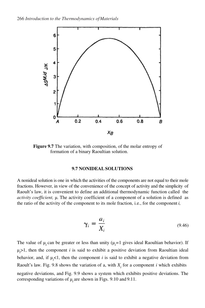
266 Introduction to the Thermodynamics ofMaterials Figure 9.7 The variation, with composition, of the molar entropy of formation of a binary Raoultian solution. 9.7 NONIDEALSOLUTIONS A nonideal solutionis one in whichthe activities ofthe componentsare not equalto their mole fractions. However, in view of the convenience of the concept of activity and the simplicity of Raoult s law, it is convenient to define an additional thermodynamic function called the activity coefficient, . The activity coefficient of a component of a solution is defined as the ratio of the activity of the component to its mole fraction, i.e., for the componenti, (9.46) The value of ican be greater or less than unity ( i=1 gives ideal Raoultian behavior). If i>1, then the component i is said to exhibit a positive deviation from Raoultian ideal behavior, and, if i<1, then the component i is said to exhibit a negative deviation from Raoult s law. Fig. 9.8 shows the variation of a, with Xifor a component i which exhibits negative deviations, and Fig. 9.9 shows a system which exhibits positive deviations. The corresponding variations of iare shown in Figs. 9.10 and9.11.

The Behavior of Solutions 267 If i varies with temperature,then has a nonzero value, i.e., from Eq.(9.41) Figure 9.8 Activities in the system iron-nickel at 1600 C. (From G.R.Zellars, S.L.Payne, J.P.Morris, and R.L.Kipp, The Ac- tivities of Iron and Nickel in Liquid Fe-Ni Alloys, Trans. AIME (1959), vol. 215, p. 181.)

268 Introduction to the Thermodynamics ofMaterials Figure 9.9 Activities in the system iron-copper at 1550 C. (From J.P.Morris and G.R.Zellars, Vapor Pressure of Liquid Cop- per and Activities in Liquid Fe-Cu Alloys, Trans. AIME (1956), vol. 206, p. 1086.) Figure 9.10 Activity coefficients in the system iron-nickel at 1600 C.

The Behavior of Solutions 269 Figure 9.11 Activity coefficients in the system iron-copper at 1550 C. and Thus andas then (9.47)

270 Introduction to the Thermodynamics ofMaterials In general, increasing the temperature of a nonideal solutions causes a decrease in the extent to which its components deviate from ideal behavior, i.e., if i>1 then an increase in temperature causes ito decrease toward unity, and if i<1 an increase in temperature causes ito increase toward unity. Thus in a solution, the components of which exhibit positive deviations from ideality, the values of the activity coefficients decrease with increasing temperature, and hence, from Eq. (9.47), the partial molar heats of solution of the components are positive quantities. Thus OHM, the molar heat of formation of the solution is a positive quantity, which indicates that the mixing process is endothermic. OHMis the quantity of heat absorbed from the thermostatting heat reservoir surrounding the solution per mole of solution formed at the temperature T. Conversely, in a solution, the components of which exhibit negative deviations from ideality, the activity coefficients increase with increasing temperature, and hence, the partial molar heats of mixing and the molar heat of mixing are negative. Such a solution forms exothermically, and OHMis the heat absorbed by the thermostatting heat reservoir, per mole of solution formed, at the temperature T. Exothermic mixing in an A B binary system occurs when the A B bond energy is more negative than both the A A and B B bond energies, and this causes a tendency toward ordering in the solution, in which the A atoms attempt to only have B atoms as nearest neighbors and vice versa. Exothermic mixing thus indicates a tendency toward the formation of a compound between the two components. Conversely, endothermic mixing occurs when the A B bond energy is less negative than both the A A and B B bond energies, and this causes a tendency toward phase separation or clustering in the solution. The A atoms attempt to be coordinated only by A atoms, and the B atoms attempt to be coordinated only by B atoms. In both cases the equilibrium configuration of the solution is reached as a compromise between the enthalpy factors, which, being determined by the relative magnitudes of the bond energies, attempt to either completely order or completely unmix the solution, and the entropy factor which attempts to maximize the randomness of mixing of the atoms in the solution. 9.8 APPLICATION OF THE GIBBS-DUHEM RELATION TOTHE DETERMINATION OF ACTIVITY As was stated in Sec. 9.4, it is often found that the activity of only one component of a binary solution can be measured experimentally. In such cases the variation of the activity of the other component can be obtained from an application of the Gibbs-Duhem equation, Eq. (9.20),

The Behavior of Solutions 271 Applied to a binary A B solution and using Gibbs free energy as the extensive property, Eq. (9.20) becomes (9.48) and, as ln ai, then (9.49) or (9.50) If the variation of aB with composition is known, then integration of Eq. (9.50) from XA=1 to XA gives the value of log aA at XAas (9.51) As an analytical expression for the variation of the activity of B is not usually computed, Eq. (9.51) is solved by graphical integration. Fig. 9.12 shows a typical variation of log aB with composition, and the value of log aA at XA=XA is equal to the shaded area under the curve. Two points are to be noticed in Fig. 9.12: 1. As XB 1, aB 1, log aB 0, and XB/XA . Thus the curve exhibits a tail to infinity as XB 1. 2. As XB 0, aB 0, and log aB . Thus the curve exhibits a tail to minus infinity as XB 0. Of these two points, point 2 is the more serious, as the calculation of log aAat any composition involves the evaluation of the area under a curve which tails to minus infinity. This introduces an uncertainty into the calculation. The tail to minus infinity can be eliminated by considering activity coefficients instead of activities in the Gibbs-Duhem equation. In the binary A B solution

272 Introduction to the Thermodynamics ofMaterials Thus (9.52) Therefore Figure 9.12 A schematic representation of the variation of log aBwith XB/XAin a binary solution, and illustration of the application of the Gibbs-Duhem equation to calculation of the activity of component A. or (9.53) Subtraction of Eq. (9.53) from Eq. (9.49) gives

The Behavior of Solutions 273 or (9.54) Thus, if the variation of B with composition is known, then integration of Eq. (9.54) gives the value of log A at the composition XA=XAas (9.55) A typical variation of log Bwith composition in a binary A B solution is shown in Fig. 9.13. The value of log A at XA=XA is given as the shaded area under the curve between the limits log B at XA=XA and log B atXA=1. Figure 9.13 A schematic representation of the variation of log B with XB/XA in a binary solution, and illustration of the application of the Gibbs-Duhem equation to calculation of the activity coefficient of component A.

274 Introduction to the Thermodynamics ofMaterials The a-Function The second tail to infinity is eliminated by the introduction of the a-function, which for the component i is defined as (9.56) The a-function is always finite by virtue of the fact that i 1 as Xi 1. For the components of a binary A B solution or (9.57) Differentiation of ln gives (9.58) and substitution of Eq. (9.58) into Eq. (9.54)gives (9.59) Integration of Eq. (9.59)gives (9.60) By virtue of theidentity

The Behavior of Solutions 275 the second integral on the right-hand side of Eq. (9.60) can be written as substitution of which into Eq. (9.60)gives (9.61) Thus ln Aat XA=XAis obtained as XBXAaBminus the area under the plot of aBvs. XA from XA=XA to XA=1, and, as aB is everywhere finite, the integration does not involve a tail to infinity. Fig. 9.8 shows the variation of aNiwith composition in the system Fe-Ni at 1600 C as measured by Zellars et al.,* and Fig. 9.10 shows the corresponding variation of Ni with composition. Extrapolation of Ni to XNi=0 in Fig. 9.10 gives the value of the Henry slaw constant (k in Eq. (9.14)) as 0.66 for Ni in Fe at 1600 C. This, then, is the slope of the Henry s law line for Ni in Fe drawn in Fig. 9.8. The variation of Fewith composition, shown in Fig. 9.10, is determined from consideration of either Fig. 9.14 or Fig 9.16. Fig. 9.14 shows the variation of log which, according t o Eq. (9.55), gives the variation of log Fe with composition. with XNi/XFe, graphical integration of Ni *G.R.Zellars, S.L.Payne, J.P.Morris, and R.L.Kipp, The Activities of Iron and Nickel in Liquid Fe-Ni Alloys, Trans. AIME (1959), vol. 215, p. 181.

276 Introduction to the Thermodynamics ofMaterials Figure 9.14 Application of the Gibbs-Duhem equation to determination of the activity of iron in the systemiron-nickel. Figure 9.15 Application of the Gibbs-Duhem equation to determination of the activity of iron in the systemiron-copper.

The Behavior of Solutions 277 Figure 9.16 The variation of aNi with composition in the system iron-nickel. In the graphical integration, as log integrated area under the curve between XNi=XNi and XNi=0 is a positive quantity. Thus log Feis everywhere a negative quantity, and so Fe, like Ni, exhibits negative deviations from Raoult s law. The variation of aNiwith composition is shown in Fig. 9.16. As aNiis everywhere negative, the integrated area from XFe=XFeto XFe=1 is a positive quantity. Fig. 9.9 shows the variation of aCuwith composition in the Fe-Cu system at 1550 C measured by Morris and Zellars.* Fig. 9.11 shows the corresponding variation of Cuwith composition. Extrapolation of Cuto XCu=0 gives kCu=10.1.Figures 9.15 and 9.17, respectively, show plots of log Cuvs. XCu/XFeand aCuvs. XFe. As log Cu decreases with increasing XCu/XFe, and aCuis everywhere positive, the integrated areas in both figures are negative quantities. increases with increasing XNi/XFe, the Ni The Relationship between Henry s and Raoult s Laws Henry s law for the solute B in a binary A B solution is or, in terms oflogarithms, *J.P.Morris and G.R.Zellars, Vapor Pressure of Liquid Copper and Activities in Liquid Fe-Cu Alloys, Trans. AIME (1956). vol. 206, p. 1086.

278 Introduction to the Thermodynamics ofMaterials differentiation of which gives Figure 9.17 The variation of aCu with composition in the system iron-copper. Inserting this into the Gibbs-Duhem equation, Eq. (9.49), gives Integration gives or

The Behavior of Solutions 279 But, by definition, ai=1 when Xi=1, and thus the integration constant equals unity. Consequently, in the range of composition over which the solute B obeys Henry s law, the solvent A obeys Raoult s law. Direct Calculation of the Integral Molar Gibbs Free Energy of Mixing Eq. (11.33b) gave gives Rearranging and dividingby or Integrating between XA=XA and XA=0 gives (9.62) and, as ln aA, the integral molar Gibbs free energy of mixing of A and B can be obtained directly from the variation of aA with composition as (9.63) The measured activities of Ni in Fe and Cu in Fe shown in Figs. 9.8 and 9.9 can be used to obtain and

280 Introduction to the Thermodynamics ofMaterials The graphical integrations of these equations are shown in Fig. 9.18, in which line (a) is vs. XCu and line (c) is (ln X )/(1 X )2with X , which is the variation of the function for a component i which exhibits Raoultian behavior. As is seen, some uncertainty is introduced into the integration by virtue of the fact that the function (ln ai)/(1 Xi) as Xi 0. In Fig 9.18 the shaded area (which is the value of the integral between XCu=0.5 and XCu=0), multiplied by the factor 2.303 8.3144 1823 0.5, gives the value of OGM at X =0.5. vs. XNi. Line (b) shows the variation of i i i 2 Fe Figure 9.18 Illustration of the direct calculation of the integral molar Gibbs free energies of mixing in the systems iron-copper at 1550 C and iron-nickel at1600 C.

The Behavior of Solutions 281 The variations of OGM obtained from the graphical integrations are shown in Fig. 9.19. Applied to a solution which exhibits Raoultian behavior (line b), the integrationgives OGM = = = in agreement with Eq. (9.34). The uncertainty caused by the infinite tail as X 0 is eliminated if the equation is used the calculate the excess Gibbs free energy (see Sec. 9.9). Eq. (9.62) is a general equation Figure 9.19 The integral molar Gibbs free energies of mixing in the systems iron-copper at 1550 C and iron-nickel at 1600 C.

282 Introduction to the Thermodynamics ofMaterials which relates the integral and partial molar values of any extensive thermodynamic function, e.g., (9.64) and (9.65) 9.9 REGULAR SOLUTIONS Thus far two classes of solution have been identified: R 1. Ideal or Raoultian solutions inwhich ln Xi 2. Nonideal solutions in which ai Xiand Attempts to classify nonideal solutions have involved the development of equations that describe the behavior of hypothetical solutions, and the simplest of these mathematical formalisms is that which generates what is known as regular solution behavior. In 1895 Margules* suggested that, at constant temperature, the activity coefficients, A and B, of the components of a binary solution could be represented by power series of the form (9.66) and, by application of the Gibbs-Duhem equation,namely, (9.54) he showed that if these equations are to hold over the entire range of composition of the solution, then a1= 1=0. This is proved by obtaining both sides of Eq. (9.54) as power series of XA and XB and equating the coefficients. By such comparison of the coefficients of the power series, Margules further demonstrated that if the variations of the activity coefficients can be represented by the quadratic terms alone, then (9.67) *M.Margules ber die Zusammensetzung der ges ttigten Dampfe von Mischungen, Stizungsberichte. Akad. Wiss. Vienna (1895), vol. 104, p. 1243.

The Behavior of Solutions 283 In 1929 Hildebrand, using an equation of van Laar which is based upon the van der Waals equation of state for mixtures, showed that if the value of the van der Waals b is the same for both components, then, in the binary A B solution, and (9.68) Hildebrand assigned the term regular solution to one obeying Eq. (9.68). Consideration of Eq. (9.61) shows that if the value of a for one component, say, component B, is independent of composition, then But, as Eq. (9.57) gave ln , it is seenthat From Eq. (9.68), a for a regular solution is an inverse function of temperature,i.e., (9.69) J.H.Hildebrand, Solubility XII, Regular Solutions, J. Am. Chem. Soc. (1929), vol. 51, p.66. J.J.van Laar, The Vapor Pressure of Binary Mixtures, Z. Physik. Chem. (1910), vol. 72, p. 723.

284 Introduction to the Thermodynamics ofMaterials Hildebrand defined a regular solution as one in which The properties of a regular solution are best examined by means of the concept of excess functions. The excess value of an extensive thermodynamic solution property is simply the difference between its actual value and the value that it would have if the solution were ideal, e.g., as applied to the Gibbs free energy of the solution. (9.70) where G=the molar Gibbs free energy of the solution Gid=the molar Gibbs free energy which the solution would have if it were ideal GXS=the excess molar Gibbs free energy of the solution Subtraction of the Gibbs free energy of the unmixed components both sides of Eq. (9.70) gives from (9.71) As for anysolution, and, for an idealsolution, then (9.72) For a regular solution, OSM=OSM,id, andthus (9.73)

The Behavior of Solutions 285 Now andas then (9.74a) (9.74b) For a regular solution, ln (9.74a) gives , and ln , substitution of which into Eq. (9.75) or, from Eq (9.69),gives (9.76) It is thus seen that GXS for a regular solution is independent of temperature. This can also been shown as follows: and, as SXS for a regular solution is zero, then GXS, and hence OHM, are independent of temperature. From Eqs. (9.74a), (9.74b), and (9.75), at any given composition,

286 Introduction to the Thermodynamics ofMaterials and hence, for a regular solution, Eq. (9.77) is of considerable practical use in converting activity data for a regular solution at one temperature to activity data at another temperature. Figs. 9.20 and 9.21, respectively, show the symmetrical variation, with composition, of the activities and activity coefficients in the system tin-thallium measured by Hildebrand and Sharma* at three temperatures, and Fig. 9.22 shows the linear variations of log T1 Figure 9.20 Activities in the system thallium-tin. (From J.H.Hildebrand and J.N. Sharma, The Activities of Molten Alloys of Thallium with Tin and Lead, J. Am. Chem. Soc. (1929), vol. 51, p. 462.) *J.H.Hildebrand and J.N.Sharma, The Activities of Molten Alloys of Thallium with Tin and Lead, J. Am. Chem. Soc. (1929), vol. 51, p. 462.

The Behavior of Solutions 287 Figure 9.21 Activities coefficients in the system thallium-tin. (From J.H.Hilde-brand and J.N.Sharma, The Activities of Molten Alloys of Thallium with TinandLead, J. Am.ChemSoc.(1929),vol.51,p.462.) Figure 9.22 Log T1 vs. and J.N.Sharma, The Activities of Molten Alloys of Thallium with Tin and Lead, J. Am. Chem. Soc (1929), vol. 51, p. 462.) in the system thallium-tin. (From J.H.Hildebrand where, the slopes of which equal a at the given temperatures. The variation of iwith Xiis that of a regular solution, but Fig. 9.23 shows that aT, which for strict adherence to regular behavior should be independent of T, decreases slowly with in- creasing temperature. Fig. 9.24 shows the variations, with composition, of OGM, OHM,

288 Introduction to the Thermodynamics ofMaterials and TOSMfor the system T1 Sn 414 C. It is to be noted that a parabolic form for OHM, or GXSshould not be taken as being a demonstration that the solution is regular, as it is frequently found that GXSor OHMcan be adequately expressed by means of the relations where b and b are unequal, in which case from Eq.(9.72) This type of behavior is found in melts in the system Au Cu and Au Ag. In the system Au-Cu at 1550 K,GXS= 24,060 X X joules is parabolic, OHMis asymmetric, and Cu iAu SXS 0. Conversely, in the system Au Ag at 1350 K, OHM= 20,590 X X joules is Ag Au parabolic, GXS is asymmetric, and SXS 0. The molar excess Gibbs free energy can be obtained from a knowledge of the dependence, on composition, of the activity coefficient of one component by means of Eq. (9.63), written as XS Thus, for a Raoultian solutions, as A=1, G =0, and for a regular solution, as ln . Figure 9.23 The variation of the product aT with T in the system T1 Sn.

The Behavior of Solutions 289 Figure 9.24 The molar enthalpy, entropy, and Gibbs free energy of mixing of thallium and tin at414 C. 9.10 ASTATISTICALMODELOF SOLUTIONS Regular solution behavior can be understood by application of the statistical mixing model, introduced in Chap. 4, to two components which have equal molar volumes and which do not exhibit a change in molar volume when mixed. In both the pure state and in solution the interatomic forces exist only between neighboring atoms, in which case the energy of the solution is the sum of the interatomic bond energies. Consider 1 mole of a mixed crystal containing NAatoms of A and NBatoms of B such that where NO is Avogadro s number. The mixed crystal, or solid solution, contains three types of atomic bond: 1. A A bonds the energy of each of which is EAA