Actuarial Reserving Strategies: Understanding Unearned Premium Reserves

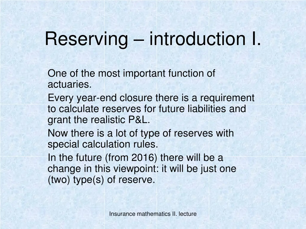
Reserving introduction I. One of the most important function of actuaries. Every year-end closure there is a requirement to calculate reserves for future liabilities and grant the realistic P&L. Now there is a lot of type of reserves with special calculation rules. In the future (from 2016) there will be a change in this viewpoint: it will be just one (two) type(s) of reserve. Insurance mathematics II. lecture

Reserving introduction II. Legal regulation: 8/2001 Ministry of Finance Regulation Requirement: all reserves have to calculate per business lines (not per products) Reserves are important because of measure also (total reserves are about 2.000 billion HUF at 2013). Insurance mathematics II. lecture

Unearned premium reserve I. Example: we take out a household policy at 01.12.2014 with 24.000 HUF yearly premium. We agree yearly payment frequency and we pay total premium in December. What is the realistic P&L situation at 31.12.2014? 30.11.2015 01.12.201431.12.2014 2.000 HUF HUF HUF 2.000 2.000 22.000 HUF 22.000 HUF Insurance mathematics II. lecture

Unearned premium reserve II. Suppose that no any claim related to this policy. What is the real P&L figure in 2014 and 2015? - If we would book whole premium for 2014 then we would not book any premium for 2015, but we are in risk during 11 months! But we got really the whole premium in 2014. The solution: 1. We book whole premium for 2014. 2. We calculate unearned premium reserve for 2014. It means that this part of premium will be the offset of risk in 2015. The value of UPR is: 11 = 24 000 . 22 000 . HUF 12 Insurance mathematics II. lecture

Unearned premium reserve III. Generalizing: Let it be d the premium due to payment frequency; T the duration of the payment which continues into next year; K the duration till date of year-closure, then: T K = UPR d T Insurance mathematics II. lecture

Unearned premium reserve IV. Open problems with this definition: -the lengths of months are not equal (in the example the real UPR is not 21.962 HUF ?); - the risk can be not equal in the whole period (example: fleets); - based on Hungarian regulation it should not reserve UPR more then 1 year; - difference between Hungarian and international regulation. The base of UPR is the yearly premium in international standard, but the payment regarding frequency in Hungarian regulation. Insurance mathematics II. lecture

Mathematical reserve Now we are dealing with mathematical reserve in non-life insurance, i.e. related to liability insurance and accident insurance. (Apart from these types there are mathematical reserve regarding life insurance and health insurance also.) Insurance mathematics II. lecture

Mathematical reserve in liability insurance I. This type is used generally if the insurer has to pay annuity based on liability insurance (typically in Hungary MTPL). The total future annuity payments are estimated with the next formula: 1 b d S i l k x + = l 1 n = 1 ( + + + x k ( ) ) MR k k 1 ( ) 0 where: -x is an age of annuitant; - lxcomes from mortality table (number of x ages); - n is the unexpired years regarding annuity; - Sk is the yearly annuity in the k-th year (with taxes); Insurance mathematics II. lecture

Mathematical reserve in liability insurance II. - i is the technical interest (the yield which the insurer will reach till end of annuity with guarantee; now based on the regulation the maximum of technical interest is 0 according to liability insurance); - d,b are cost factors; typically one of them is 0. If there is an L limit in the policy related to annuity the formula will change as follows: MR = * min( , ) L MR Insurance mathematics II. lecture

Mathematical reserve in liability insurance III. The formula is uncomplicated, but the estimation of parameters is not easy: - in the most cases the insurer knows just the initial annuity. In the long run it can be a lot of change regarding the health status of annuitant, inflation, etc.; -the mortality of annuitant is different comparing the total mortality rate (but there are no separate mortality table of annuitant). It can cause unexpected profit or loss. Because of above reasons the insurer usually tends to pay lump sum (typically 50-60% of virtual mathematical reserve). Insurance mathematics II. lecture

Mathematical reserve in accidental insurance The formula is similar as in liability insurance, but the change of annuity is not so frequent because usually the measure of annuity is exact in the policy. Insurance mathematics II. lecture

Claims reserve I. Reasons: - lag in reporting of claims; - lag in payment of claims. There are two types of claims reserve: -If the insurer has known the claims but the claims are not totally payed, there are Outstanding Claims Reserve (OS Reserve); -If the insurer has not yet known the claims, it can be used IBNR reserve (incurred but not reported). Insurance mathematics II. lecture

Claims reserve II. There are two different possible approach: - separate assumption for OS and IBNR reserve or - together estimating with statistical methods. Now in Hungary it is used the separate approach generally, but because of Solvency II. in the future the second approach will come into view. The measure of lag is characteristic for products, for example the CASCO and accident products have usually higher speed run-off, and MTPL and other liability products have usually slower run-off. Insurance mathematics II. lecture

Claims reserve III. For assumption it can consider inflation and the yield of reserves also. It is interesting and generally unanswerable question how is the most useful splitting of portfolio for the assumption: The target is to find homogenous groups of risks. It can be per products or per business lines or sometimes in one product there is useful to further splitting (for example, in MTPL splitting between annuities and non- annuities, or splitting big claims and non-big claims). Insurance mathematics II. lecture

Outstanding claims reserve and claims handling reserve In separate OS reserve assumption methods the actuaries have no a lot of tasks. The claim experts have experience how much can be the best estimate of the different claim event. The actuaries have just one task: calculate claims handling reserve with the next formula: CHP = CHR CLR where CP CHR claims handling reserve; CHP claims handling payment in current year; CP claims payment in current year; CLR claims reserve (OS or IBNR). Insurance mathematics II. lecture

IBNR reserve I. There are a lot of different algorithm to evaluate IBNR reserve. Before the detailed description of these methods it can be useful to define several basic ideas. Reporting/payment year .. X, 1 X n 1 , 1 .. X, Accident year Run-off triangles i j X, means the total amount of claims which are occurred in i-th year and reported/paid in j-th year i j X 1 , n Insurance mathematics II. lecture

IBNR reserve II. Development year .. X X, 1 1 , 1 n Accident year Lagging triangles .. X, i j X, means the total amount of claims which are occurred in i-th year and reported/paid in (i+j-1)-th year i j X 1 , n Insurance mathematics II. lecture

IBNR reserve III. Development year .. X X, 1 1 , 1 n Accident year Cumulated triangles .. X, i j X, means the total amount of claims which are occurred in i-th year and reported/paid till (i+j-1)-th year i j X 1 , n Insurance mathematics II. lecture

IBNR reserve IV. The cumulated triangle is complete, if there is no any reporting/paying after n-th year (difficult to say). It is possible to make run-off triangles for number of claims also. Hungarian regulation requires for IBNR calculation just using run-off triangles. For assumption the cumulated triangle will be the basic usually. Insurance mathematics II. lecture

IBNR reserve V. Denote X, the claims which are reported/paid after n-th + i n year regarding claims occurred in i-th year. Our target is estimating the next formula (for each i): X X IBNR + = 1 , , Our best estimate is as follows: + i i n i n i = + ) 1 + ( , X E X X u v n + + , , , i n i n u v Our problem is that in practice usually we do not know covariance and common distribution of claims. That is why we simplify in the methods which we are using for calculation of IBNR. Insurance mathematics II. lecture

Methods of IBNR calculation Grossing Up method I. Example: 1 2 3 4 5 Development year 2009 223; 311; 252; 127; 29 Accident year 2010 254; 378; 249; 153 2011 312; 411; 276 Lagging triangle 2012 359; 435 2013 384 Insurance mathematics II. lecture

Methods of IBNR calculation Grossing Up method II. Example: 1 2 3 4 5 Development year 2009 223; 534; 786; 913; 942 Accident year 2010 254; 632; 881; 1034 2011 312; 723; 999 Cumulated triangle 2012 359; 794 2013 384 Insurance mathematics II. lecture

Methods of IBNR calculation Grossing Up method III. Example: Is the cumulated triangle complete? No, we have data from earlier years as follows: Year Claims until 5th year Total Ratio (5th year/Total) 2005 780 830 93,98% 2006 810 890 91,01% 2007 800 860 93,02% Total 2390 2580 92,64% Insurance mathematics II. lecture

Methods of IBNR calculation Grossing Up method IV. Example: Assumption for 2009: 942 = 1017 9264 , 0 The base of assumption will be 2009 as next table shows: 1. year 2. year 3. year 4. year 5. year Total 2009 223 534 786 913 942 1017 Ratio 21,9% 52,5% 77,3% 89,8% 92,64% 100% We assume that the run-off of next years will be equal as 2009. Insurance mathematics II. lecture

Methods of IBNR calculation Grossing Up method V. Example: 1 2 3 4 5 Total IBNR 1017 75 2009 223; 534; 786; 913; 942 Occurring year 1152 118 2010 254; 632; 881; 1034 1292 293 2011 312; 723; 999 1512 718 2012 359; 794 2013 384 1751 1367 Total 2571 Insurance mathematics II. lecture

Methods of IBNR calculation Grossing Up method VI. Generalizing: X 1. Based on earlier year we estimate , 1 = n d n X + , 1 n If we have no any data from earlier year we can use data from similar products or OS reserves. X X X 2. Further factors: . , 1 1 , 1 2 = 1 = 2 1 , 1 = n n d d d X X X 1 n n + + + , 1 , 1 , 1 n n n 3. Ultimate payment estimation: X X X . , 3 2 1 , n += = n , 2 1 += n X X X + , 3 , n n n , 2 n d d d 2 1 n 1 n Insurance mathematics II. lecture

Methods of IBNR calculation Grossing Up method VII. 4. Reserve assumption: X = ; 1 V X i n + + , , 1 i i n i = i n i n = V iV 1 The above calculation is the basic version, but there are some modified possibility of this method. Insurance mathematics II. lecture

Methods of IBNR calculation Modified Grossing Up methods I. 1. version: If we have data related to earlier year splitting per year then we can calculate more exact the d factors. X d i = + , 1 Let and , 1 1 i ( 1 ), ( ),..., 2 ( ); 1 d d d k i n ) 1 ( ; 1 i n X i i i n the other experience d factors. Then the ultimate used factors: + + 1 + + ) 1 ( ( ) 1 ( ) 2 ... ( ) d d d d k = ; 1 i i i + i d i n i k Insurance mathematics II. lecture

Methods of IBNR calculation Modified Grossing Up methods II. Example: 1. year 2. year 3. year 4. year 5. year Total 2005 Ratio (%) 170 20,5% 422 50,8% 660 79,5% 750 90,4% 780 94% 830 100% 2006 Ratio (%) 140 15,7% 435 48,9% 680 76,4% 782 87,9% 810 91% 890 100% 2007 Ratio (%) 132 15,3% 428 49,8% 670 77,9% 780 90,7% 803 93% 860 100% 2009 Ratio (%) Average ratio 223 21,9% 18,4% 534 52,5% 50,5% 786 77,3% 77,8% 913 89,8% 89,7% 942 92,7% 92,7% 1017 100% 100% Insurance mathematics II. lecture

Methods of IBNR calculation Modified Grossing Up methods III. Example: Year Total (ultimate) payment 1017 IBNR 2009 75 2010 1153 119 2011 1284 285 2012 1572 778 2013 2090 1706 Total 2964 Insurance mathematics II. lecture

Methods of IBNR calculation Modified Grossing Up methods IV. 2. version: If we have data related to earlier year splitting per year then we can calculate more exact the d factors. X d i = + , 1 Let and , 1 1 i ( 1 ), ( ),..., 2 ( ); 1 d d d k i n ) 1 ( ; 1 i n X i i i n the other experience d factors. Then the ultimate used factors: = min( 1 ( ); ( 1 ); ( );...; 2 ( )); 1 d d d d d k i n i i i i i Insurance mathematics II. lecture

Methods of IBNR calculation Modified Grossing Up methods V. Example: 1. year 2. year 3. year 4. year 5. year Total 2005 Ratio (%) 170 20,5% 422 50,8% 660 79,5% 750 90,4% 780 94% 830 100% 2006 Ratio (%) 140 15,7% 435 48,9% 680 76,4% 782 87,9% 810 91% 890 100% 2007 Ratio (%) 132 15,3% 428 49,8% 670 77,9% 780 90,7% 803 93% 860 100% 2009 Ratio (%) Minimum ratio 223 21,9% 15,3% 534 52,5% 48,9% 786 77,3% 76,4% 913 89,8% 87,9% 942 92,7% 91% 1017 100% 100% Insurance mathematics II. lecture

Methods of IBNR calculation Modified Grossing Up methods VI. Example: Year Total (ultimate) payment 1035 IBNR 2009 93 2010 1177 143 2011 1308 309 2012 1625 831 2013 2502 2118 Total 3493 Insurance mathematics II. lecture

Methods of IBNR calculation Modified Grossing Up methods VII. X 3. version: We estimate as in 1. version. After ; 1 ( 1 ); d i n + , 1 n i X it we judge ultimate payment for 2.year: , 2 1 += n X , 2 n ) 1 ( 1 d n With this result we define the d factors and estimate ultimate payment as follows: X X , 2 2 1 , 2 = = n ) 2 ( ...; ; d ) 2 ( d X X 2 1 n + + , 2 , 2 n + n ) 1 ( 2 ) 2 ( 2 d d = n n d 2 n 2 X , 3 2 += n X , 3 n d 2 n After it we continue this process till each d factors and payments will be calculated. Insurance mathematics II. lecture

Methods of IBNR calculation Modified Grossing Up methods VIII. Example: 1. year 2. year 3. year 4. year 5. year Total 2009 Ratio (%) 223 21,9% 534 52,5% 786 77,3% 913 89,8% 942 92,6% 1017 100% 2010 Ratio (%) 254 22,1% 632 54,9% 881 76,5% 1034 89,8% 1152 100% 2011 Ratio (%) 312 24% 723 55,6% 999 76,9% 1299 100% 2012 Ratio (%) 359 24,6% 794 54,3% 1461 100% 2013 Ratio (%) 384 23,1% 1659 100% Insurance mathematics II. lecture

Methods of IBNR calculation Modified Grossing Up methods IX. Example: Year Total (ultimate) payment 1017 IBNR 2009 75 2010 1152 118 2011 1299 300 2012 1461 667 2013 1659 1275 Total 2434 Insurance mathematics II. lecture

Methods of IBNR calculation Modified Grossing Up methods X. X 4. version: We estimate as in 1. version. After ; 1 ( 1 ); d i n + , 1 n i X it we judge ultimate payment for 2.year: , 2 1 += n X , 2 n ) 1 ( 1 d n With this result we define the d factors and estimate ultimate payment as follows: X X , 2 2 1 , 2 = = n ) 2 ( ...; ; d ) 2 ( d X X 2 1 n + + , 2 , 2 n n = min( 1 ( 2 ); 2 ( 2 )) d d d 2 n n n X , 3 2 += n X , 3 n d 2 n After it we continue this process till each d factors and payments will be calculated. Insurance mathematics II. lecture

Methods of IBNR calculation Modified Grossing Up methods XI. Example: 1. year 2. year 3. year 4. year 5. year Total 2009 Ratio (%) 223 21,9% 534 52,5% 786 77,3% 913 89,8% 942 92,6% 1017 100% 2010 Ratio (%) 254 22,1% 632 54,9% 881 76,5% 1034 89,8% 1152 100% 2011 Ratio (%) 312 24% 723 55,6% 999 76,5% 1306 100% 2012 Ratio (%) 359 24,6% 794 52,5% 1512 100% 2013 Ratio (%) 384 21,9% 1753 100% Insurance mathematics II. lecture

Methods of IBNR calculation Modified Grossing Up methods XII. Example: Year Total (ultimate) payment 1017 IBNR 2009 75 2010 1152 118 2011 1306 307 2012 1512 718 2013 1753 1369 Total 2587 Insurance mathematics II. lecture

Methods of IBNR calculation Link ratio methods I. X + , 1 i j = ( ) c i We suppose that ratio does not depend on significantly for i j X , i j X 1 1. Determining is similar then in the Grossing Up method. + = = , i n c n d X , n i n jc (with experience of earlier years or OS reserve). Other factors will be (i ) cj defined as function of actual . With choosing different function will be defined the different version of link ratio method. 2. Ultimate payment and IBNR reserve estimation: , 1 X = = = ) 1 X c X ( V X c X + , 1 n n n + 1 , 1 , 1 , 1 n n n n Insurance mathematics II. lecture

Methods of IBNR calculation Link ratio methods II. 2. Ultimate payment and IBNR reserve estimation: = = = ) 1 ( X c c X V X X c c X + + , 2 1 , 2 1 2 , 2 , 2 1 1 , 2 1 n n n n n n n n n = = = ) 1 ... ( ... X c c c X V X X c c c X + + , 1 1 1 , n , 1 , n 1 1 1 , n n n n n n n n n n = 1 ( j ); 1 1 c c j n Basic version: j + + + ) 1 ( j ) 2 ( j ... j ( ) c c c n j j = ; 1 1 c j n 1. modification: j n Insurance mathematics II. lecture

Methods of IBNR calculation Link ratio methods III. = max( 1 ( j ); 2 ( j );... ( )); 1 1 c c c c n j j n 2. modification: j j 3. modification: + + + ) 1 ( j ) 2 ( n ... j ( ) c c c n j , 1 , 2 , j j j n j j j = ; 1 1 c j n j In 3. modification with special factors we will get the most popular chain-ladder method. Insurance mathematics II. lecture

Methods of IBNR calculation Chain ladder method I. This is the most popular process for IBNR estimation. + + + ) 1 ( j ) 2 ( j ... ( ) X c X c X c n j , 1 , 2 , j j n j j j = = c j + + + ... X X X , 1 , 2 , j j n j j + + + ... X X X + + + , 1 1 , 2 1 , 1 j j n j j = ; 1 1 j n + + + ... X X X , 1 , 2 , j j n j j Insurance mathematics II. lecture

Methods of IBNR calculation Chain ladder method II. Example: Year Total (ultimate) payment 1017 IBNR 2009 75 2010 1152 118 2011 1300 301 2012 1458 664 2013 1648 1264 Total 2420 Insurance mathematics II. lecture

Methods of IBNR calculation Naive loss ratio method In the next methods we are using premium data also (not just claim data). i We suppose that the ultimate loss of i-th year will be the 1 -th part of the premium. Then the reserve can be calculated as follows: = 1 ( ) V P = i X + , 1 i i i i n i n iP = , where signs the earned premium of i-th year. V iV 1 The disadvantage of this method is that IBNR reserve is independent of actual claim data. Starting company without any own claim data can use this method. Insurance mathematics II. lecture

Methods of IBNR calculation Bornhuetter-Ferguson method I. This method combines the naive loss ratio and grossing up (or link ratio) methods. 1. We calculate the ultimate loss payment with naive claim ratio methods: = 1 ( ) X P + , i n i i 2. For calculating development factors we are using grossing up (or link ratio method): X c , X X 1 1 1 = = = , , 1 1 , i n i n i ; ;... d d d 1 1 n n ... X c c X c c c X + + + 1 , 1 1 , n i n n n i n n n i n Insurance mathematics II. lecture

Methods of IBNR calculation Bornhuetter-Ferguson method II. 3. The reserves will be estimated as follows: 1 X X = = 1 ( ) 1 ( ) V d + + 1 , 1 , 1 n n n c n 1 X X = = 1 ( ) 1 ( ) V d + + 2 1 , 2 , 2 n n n c c 1 n n . 1 X X = = 1 ( ) 1 ( ) V d + + 1 , , n n n n n ... c c c 1 1 n n n = i = V iV 1 Insurance mathematics II. lecture

Methods of IBNR calculation Separation method I. In this method we do not use cumulated triangles, but we are using lagging triangles. The used triangles have to be complete. We suppose that = ; 1 , X c n r i j n + , i j i j i j in where signs the number of claims in the i-th year (known), signs an inflation, c is the average claim amount. i+ j There are two types of this method: - arithmetic; - geometric. Now we consider detailed the arithmetic version. Insurance mathematics II. lecture

Methods of IBNR calculation Separation method II. n We suppose that = j = 1 jr 1 jr It means that signs the expected proportion of claims development year j without inflation effect. In this case k is the inflation factor according to first year. 1 Then we define the next formula: X , i j = = B c r + , i j j i j n i And we use the lagging triangle for these new elements as follows Insurance mathematics II. lecture

Methods of IBNR calculation Separation method III. Development year ... 1 r 2 r r c c c nr 1 2 n ... 2 1 r c c c nr 1 3 2 n Accident year .. 1 c r n After we define diagonal sums as follows: Insurance mathematics II. lecture