Adjoint Models: Forecast Error Analysis and Sensitivity Prediction
Analyzing forecast errors and predicting sensitivity is crucial in meteorology. Adjoint models offer a way to trace errors back to their source by running a simplified version of the forward model backwards in time. This process helps in understanding how errors originated and where they occurred within the model. The concept involves adjusting model parameters and initial conditions to improve forecasting accuracy.
Download Presentation

Please find below an Image/Link to download the presentation.
The content on the website is provided AS IS for your information and personal use only. It may not be sold, licensed, or shared on other websites without obtaining consent from the author.If you encounter any issues during the download, it is possible that the publisher has removed the file from their server.
You are allowed to download the files provided on this website for personal or commercial use, subject to the condition that they are used lawfully. All files are the property of their respective owners.
The content on the website is provided AS IS for your information and personal use only. It may not be sold, licensed, or shared on other websites without obtaining consent from the author.
E N D
Presentation Transcript
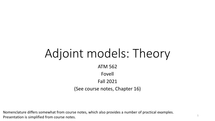
Adjoint models: Theory ATM 562 Fovell Fall 2021 (See course notes, Chapter 16) Nomenclature differs somewhat from course notes, which also provides a number of practical examples. Presentation is simplified from course notes. 1
Motivation We often look at a forecast and wonder where did this come from and how could this be changed , especially if it involves forecast error Often our strategy involves posing a hypothesis that explains the error s origin, changing the model initial conditions and/or model parameters/physics to compensate, and running the model usually over and over and over Ideally, we want an active, dynamic tracer that shows how the error came about in the model which fields, where, and when The adjoint model is a simplified and transformed version of the forward model that runs backwards The forward model predicts temperature, pressure, winds, etc., forward in time The future evolves from the past The adjoint model predicts sensitivity to temperature, pressure, winds, etc.., backwards in time Traces error back to its roots (in theory) 2
Background: simple problem 1D wave equation: M real (interior) grid points, 1 prognostic variable, 2 time level scheme c > 0 Rewrite in explicit form 3
Background: matrix form Write in matrix form (interior points j= 1, 2, , M) MxM Mx1 Mx1 For this simple problem, same B every time step. Not true for more realistic problems. Boundary condition needs to be applied (currently presuming u=0 at left side) 4
Background: integrate model Initial condition is u0. Integrate for N time steps. We can relate the final forecast to the initial condition through the transition matrix QN 5
Background: generalize model x is p prognostic fields x M interior gridpoints p 4 (i.e., u, w, , , ) M = MX x MY x MZ 6
Tangent linear model (TLM) #1 A simple model equation u = prognostic variable = model parameter Examples: 1D wave equation (parameter = -c) Exponential decay (parameter = - ) 7
Tangent linear model (TLM) #2 Run the model twice, using two different initial conditions and/or two different values for parameter . Control solution uC(x,z,t) Alternative solution uA(x,z,t) [example: warmer vs. cooler thermal] Control parameter C Alternative parameter A [example: faster vs. slower sound speed] Difference between simulations and their parameters 8
Tangent linear model (TLM) #3 You can always subtract two simulations. However, the TLM is a model that attempts to estimate the difference between the control and alternative runs, based on the control run Instead of run run calculate do this Why?We ll see run estimate TLM run 9
Tangent linear model (TLM) - example Example: Model task 0B with slightly different c or slightly shifted initial conditions Keep in mind: differences have to be small 10
Tangent linear model (TLM) #4 TLM can be formed via perturbation analysis, and as usual presumes the perturbations are (& remain) small so higher order terms can be neglected1 Uses Taylor series to approximate u if then the TLM is 11 1See course notes for qualifications and disclaimers
Tangent linear model (TLM) #5 The perturbation model has been linearized (no u term) and is constrained to ( tangent to ) the control run (uC, C). Tangent linear model Ignore for simplicity Discretize TLM and write in matrix form Cn based on control model run ONLY - Run control simulation - Archive Cn every time step (ideally) - Initialize and run TLM In this very simple example, Cn is just C and is constant every time, so no archiving is actually needed 12
Tangent linear model (TLM) #6 Integrate the TLM. Initial condition is u 0 Cn based on control model run ONLY - Run control simulation - Archive Cn every time step (ideally) - Initialize and run TLM PN is the transition matrix for TLM 13
Tangent linear model (TLM) #7 Generic form. x is p variables by M points. Initial condition is x 0 14
Forecast aspect J The forecast aspect J is something about the control run we want to examine How did some feature appear? Why did some error occur? J at time N is a scalar function of the control run at that time JN = J(xN) JN can be changed( JN) by perturbing the control run (ignoring higher order terms) 15
Change of forecast aspect JN Change of J at time N Perturbation applied to variable/location xl at time N Sensitivity of J to xl at time N p variables M locations Perturb a variable/location It only changes J if J is sensitive to it!!!! 16
Change of forecast aspect JN Let JNbe surface pressure at one point, say 30 N 60 W, at time N JN is the change in surface pressure at that place and time At time N, this JN is sensitive to only one variable and location pressure at that very location Therefore, of the p x M terms in the sum, only one sensitivity is nonzero, and it is equal to 1 Thus JN is KNOWN information and is TRIVIAL 17
Making this less trivial Renaming sensitivity for convenience Rewrite as an inner product Postulate the adjoint model, a prediction model for sensitivity x* From control run Take the TLM model and (a) Replace x by x* (b) Transpose Cn (c) Operate it backwards TLM Adjoint Note CnT Cn-1, so we are NOT running the TLM backwards ALSO, Cn cannot usually be inverted anyway (not full rank) 18
TLM vs. adjoint The control run information used to step perturbationsforward in time... ...is transposed and used to step sensitivity backwards in time 19
TLM and adjoint Relating initial and final times for TLM and adjoint models x , x* are vectors M x 1 P is a matrix M x M Next, we will make use of the adjoint property a, b are vectors M x 1 L is a matrix M x M This is how the adjoint model got its name 20
The recipe by definition trivial relate final to initial time invoke adjoint property relate final to initial time Note therefore that 21
The recipe KNOWN TRIVIAL KNOWN NOT TRIVIAL! x0* identifies which perturbations x have to be at the initial time to get that desired change to J at final time N 22
Integrating the adjoint (1) Run the control model forwards to time N and archive Cn every time step (ideally) (2) Initialize adjoint model at time N (3) Integrate adjoint model backwards, reading in Cn from archive You DON T need to integrate the TLM at all!!! 23
To summarize The control simulation is made by integrating a (likely nonlinear) model forward in time, producing forecasts of temperature, pressure, winds, etc.. The tangent linear model (TLM) is a linearized version of the forward model, producing forecasts of perturbations (deviations) from the control forecast The inescapable assumption is the deviations are small (truncated Taylor series) The adjoint model is a transposed version of the TLM The adjoint model runs backwards in time The adjoint propagates sensitivity to temperature, pressure, winds, etc., backwards It represents an active, dynamical tracer that shows how the model got to its final state It also must assume that deviations are (and remain) small Our simple examples involved differentiating the model differential equation to create the TLM. In practice, we differentiate the model code. For code with a lot of complicated physics, especially on/off switches (microphysics!!!), this is very difficult. Software exists to automate some of this. 24
Adjoint models and data assimilation Most common use for TLM/adjoint models: they are integral to 4- dimensional variational data assimilation (4D-Var) WRF-ARW system also provides a TLM and adjoint version But only a small subset of model physics have adjoint versions available Can be used to assess forecast sensitivity to observations (FSO), e.g., Zhang et al. (2015): In addition to the traditional observation-denial method, often referred to as Observation System Experiments (OSEs) the adjoint-based forecast sensitivity to observation (FSO) method is an efficient approach to assess relative observation impact on a measured aspect of the forecast error. Unlike OSEs, which measure effects of a single observation on all forecast metrics, FSO quantifies the response of a single forecast metric to all perturbations of the observing systems. It can directly assess the impact of any or all observations used by a forecasting system during data assimilation on a selected measure of short-range forecast error 25
[end] 26
