Advanced Concepts in Difference Equations: Stability, Analysis, and Applications

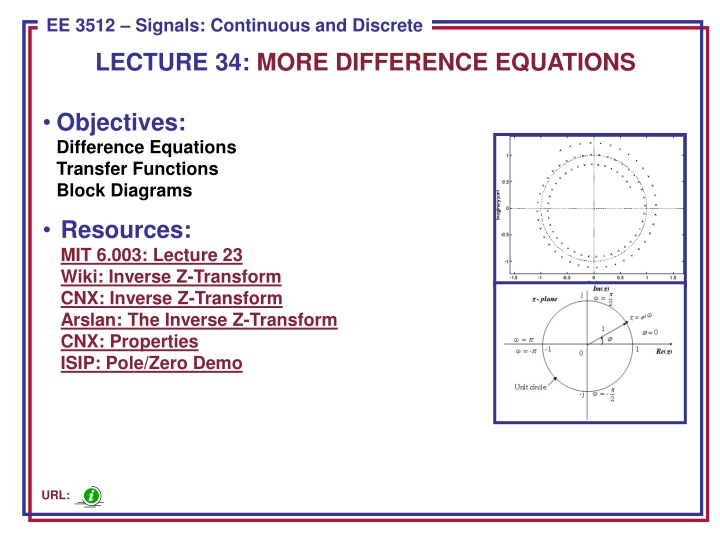
ECE 8443 Pattern Recognition EE 3512 Signals: Continuous and Discrete LECTURE 34: MORE DIFFERENCE EQUATIONS Objectives: Difference Equations Transfer Functions Block Diagrams Resources: MIT 6.003: Lecture 23 Wiki: Inverse Z-Transform CNX: Inverse Z-Transform Arslan: The Inverse Z-Transform CNX: Properties ISIP: Pole/Zero Demo URL:

First-Order Difference Equations Consider a first-order difference equation: ] [ ] 1 [ ] [ n bx n ay n y = + We can apply the time-shift property: ) ( ) ( y z Y z a z Y + + ] 1 = 1 [ ( ) bX z We can solve for Y(z): ay z Y + [ az ] 1 b = + ( ) ( ) X z + 1 1 1 1 az The response is again a function of two things: the response due to the initial condition and the response due to the input. If the initial condition is zero: b z Y ( ) Y z b = = = ( ) ( ) ( ) X z H z + + 1 1 ( ) X z 1 1 az az Applying the inverse z-Transform: b n h + = = 1 n Z [ ] ( ) [ ] b a u n 1 1 az Is this system causal? Why? Is this system stable? Why? Suppose the input was a sinusoid. How would you compute the output? EE 3512: Lecture 34, Slide 1

Example of a First-Order System Consider the unit-step response of this system: 1 z = = = [ ] [ ] ( ) x n u n X z 1 z a 1 z ] 1 az ] 1 az [ [ 1 ay b ay b = + = + ( ) ( ) Y z X z + + + + 1 1 1 1 1 1 ay 1 1 1 1 az az z 2 [ ] 1 + z bz = + + ) 1 ( )( z a z a z Use the (1/z) approach for the inverse transform: + a + 2 ( z ) 1 z /( z 1 + ) /( z 1 ) V z bz ab a b a = = + + ) 1 ab ( )( 1 z a z + + [ ] 1 + /( z 1 + ) /( 1 z ) [ ] 1 + ay z a z b a z ay z b az z = + + = + + ( ) Y z + + 1 1 1 z a a z a a z a z b = + ) 1 ( + n n n [ ] [ 1 ]( ) [ ( ) ] y n ay a a a + b 1 a + = + + = 1 n n [ 1 ]( ) [ ( ) 1 ], , 1 , 0 , 2 ... ay a a n + 1 a The output consists of a DC term, an exponential term due to the I.C., and an exponential term due to the input. Under what conditions is the output stable? EE 3512: Lecture 34, Slide 2

Second-Order Difference Equations Consider a second-order difference equation: [ ] 1 [ ] [ 2 1 + + n y a n y a n y = + ] 1 ] 2 [ ] [ b x n b x n 0 1 We can apply the time-shift property: ) ( ) ( 1 z Y z a z Y + + ] 1 + + ] 1 + ] 2 = + 1 2 1 1 [ ( ) [ [ ( ) ( ) y a z Y z z y y b X z b z X z 2 0 1 Assume x[-1] = 0 and solve for Y(z): ] 2 [ ) ( a + + ] 1 1 1 [ ] 1 + [ b b z a y a y a y z = + 0 1 + 2 1 2 ( ) Y z X z + 1 2 1 2 1 1 z a z a z a z 1 2 1 2 Multiplying z2/z2: ( ) + ] 1 + ] 1 2 2 [ [ a ] 2 z [ b z b + z a y a y z a y z = + 0 + 1 1 2 + 2 ( ) ( ) Y z X z + 2 2 z a z a z a 1 2 1 2 Assuming the initial conditions are zero: z b z b z Y + + + 2 = 0 1 ( ) 2 z a z a 1 2 Note that the impulse response is of the form: ( ] [ cos ] [ n u n a n h = 2 ) ( cos ) z a z + = n ( ) H z 2 ( 2 2 cos ) z a z a This can be visualized as a complex pole pair with a center frequency and bandwidth (see Java applet). EE 3512: Lecture 34, Slide 3

Example of a Second-Order System Consider the unit-step response of this system: 1 z = = = [ ] [ ] ( ) x n u n X z 1 z a 1 z 5 . 1 + ] 1 5 . 0 + = ] 1 ] 1 = ] 2 = [ ] [ [ ] 2 ) + [ ] [ where [ , 2 [ 1 y n y ( a n y n x n x n y y + z ] 1 + z ] 2 z a ] 1 2 2 [ [ [ b z b z y a y z a y z = + 0 + 1 1 2 + 2 ( ) ( ) Y z X z + 2 2 a z a a 1 2 1 2 ( 5 . 1 ( ) + z 5 . 0 ( 2 2 ) 2 )( 5 . 0 ( 2 ) 1 )( z ) 2 )( z z z z z = + 5 . 1 + 5 . 0 + 5 . 1 + + 2 1 z 5 . 0 z z 5 . 3 2 2 z z z = + = 2 2 [ note ( : ) ( 1 )] z z z z z 5 . 1 + + 5 . 1 + + 2 2 5 . 0 5 . 0 z z z z We can further simplify this: = z MATLAB: num = [1 -1 0]; den = [1 1.5 .5]; n = 0:20; x = ones(1, length(n)); zi = [-1.5*2-0.5*1, -0.5*2]; y = filter(num, den, x, zi); 2 5 . 2 z z ( ) Y z 5 . 1 + z 5 . 0 + z 2 z 5 . 0 z 3 = 5 . 0 + + 1 z The inverse z-transform gives: ) 5 . 0 ( 5 . 0 ] [ = n y ) 1 = n n ( 3 , , 1 , 0 , 2 ... n EE 3512: Lecture 34, Slide 4

Nth-Order Difference Equations Consider a general difference equation: = i 1 N M = i + = [ ] [ ] [ ] y n a y n i b x n i i i 1 We can apply the time-shift property once again: N M + = i i ( ) ( ) ( ) (assuming zero initial conditions ) Y z a z Y z b z X z i i = = 1 1 i i + 1 N M = i i ( ) ( ) Y z a z X z b z i i = = 1 1 i i M i b z + + 1 + 2 + ... i 1 2 M ... b + b + z b + z b + z ( ) Y z = = = = 1 0 1 2 i M ( ) H z + N N ( ) X z 1 a a z a z a z + i 1 a z 0 1 2 N i = 1 i We can again see the important of poles in the stability and overall frequency response of the system. (See Java applet). Since the coefficients of the denominator are most often real, the transfer function can be factored into a product of complex conjugate poles, which in turn means the impulse response can be computed as the sum of damped sinusoids. Why? The frequency response of the system can be found by setting z = ej . EE 3512: Lecture 34, Slide 5

Transfer Functions In addition to our normal transfer function components, such as summation and multiplication, we use one important additional component: delay. = ] 1 [n x ] [ ] [ y n x n D = ] 1 [n x ] [ ] [ y n x n z-1 This is often denoted by its z-transform equivalent. = 1 ( ) ( ) Y z z X z We can illustrate this with an example (assume initial conditions are zero): EE 3512: Lecture 34, Slide 6

Transfer Function Example Redraw using z-transform: Write equations for the behavior at each of the summation nodes: ) ( ) ( 2 1 Y z Q z zQ + = = + ( ) zQ z Q z X z = ( ) ( z ) 3 ( z ) z 2 z 1 ( ) 2 ( ) ( ) Y Q Q 1 2 Three equations and three unknowns: solve the first for Q1(z) and substitute into the other two equations. ) ( ) ( ) ( 2 1 + = z Y z X z z Q z z zQ = + 1 1 Q z z Q z z X z z 1 1 ( ) ( ) ( ) 3 ( ) 2 2 = + 2 2 1 ( ) ( ) ( ) 3 ( ) Q z Q z z X z z Y z 2 2 1 = 2 1 ( ) ( ) 3 ( ) Q z z X z z Y z 2 2 1 z 1 1 = + + 1 2 1 1 2 1 ( ) 2 ( ) 3 ( ) 2 ( ) ( ) 3 ( ) Y z z z X z z Y z z X z z X z z Y z 2 2 1 1 z z Simplify.. . + z ( ) 2 + 1 + Y z z = = ( ) H z 2 ( ) X z 3 5 z EE 3512: Lecture 34, Slide 7

Basic Interconnections of Transfer Functions EE 3512: Lecture 34, Slide 8

Summary Demonstrated the solution of Nth-order difference equations using the z-transform: general response is an exponential. Demonstrated how to develop and decompose signal flow graphs using the z-transform: introduced a component, the delay, which is equivalent to differentiation in the s-plane. EE 3512: Lecture 34, Slide 9