Advanced Concepts in Machine Learning and Pattern Recognition

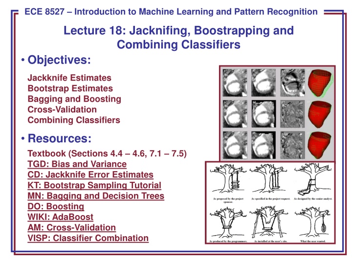
ECE 8443 Pattern Recognition ECE 8527 Introduction to Machine Learning and Pattern Recognition Lecture 18: Jacknifing, Boostrapping and Combining Classifiers Objectives: Jackknife Estimates Bootstrap Estimates Bagging and Boosting Cross-Validation Combining Classifiers Resources: Textbook (Sections 4.4 4.6, 7.1 7.5) TGD: Bias and Variance CD: Jackknife Error Estimates KT: Bootstrap Sampling Tutorial MN: Bagging and Decision Trees DO: Boosting WIKI: AdaBoost AM: Cross-Validation VISP: Classifier Combination

No Free Lunch Theorem (Review) A natural measure of generalization is the expected value of the error given D: ? ? ? = ? ? 1 ? ? ? , (?) ?( ?)?(? ?) ,? ? ? where ?() denotes the Kronecker delta function (value of 1 if the two arguments match, a value of zero otherwise). The expected off-training set classification error when the true function ?(?) and the probability for the ?? candidate learning algorithm is ??( (?) ?) is: ??? ?,? = ? ?? ? 1 ? ? ? , (?)??( (?) ?) No Free Lunch Theorem: For any two learning algorithms ?1( ?) and ?2( ?), the following are true independent of the sampling distribution?(?)and the number of training points: 1. Uniformly averaged over all target functions, ?, ?1(? ?,?) ?2(? ?,?) = 0. 2. For any fixed training set ?, uniformly averaged over ?, ?1(? ?,?) ?2(? ?,?) = 0. 3. Uniformly averaged over all priors ?(?),?1(? ?,?) ?2(? ?,?) = 0. 4. For any fixed training set ?, uniformly averaged over ?(?), ?1(? ?,?) ?2(? ?,?) = 0. ECE 8527: Lecture 18, Slide 1

Bias and Variance (Review) Two ways to measure the match of alignment of the learning algorithm to the classification problem involve the bias and variance. Bias measures the accuracy in terms of the distance from the true value of a parameter high bias implies a poor match. Variance measures the precision of a match in terms of the squared distance from the true value high variance implies a weak match. For mean-square error, bias and variance are related. Consider these in the context of modeling data using regression analysis. Suppose there is an unknown function ?(?) which we seek to estimate based on ? samples in a set ? drawn from ?(?). The regression function will be denoted ?(?;?). The mean square error of this estimate is: ?? ? ?;? ?(?)2= ??? ?;? ?(?) The first term is the bias and the second term is the variance. ?+ ?? ? ?;? ??? ?;? ? This is known as the bias-variance tradeoff since more flexible classifiers tend to have lower bias but higher variance. ECE 8527: Lecture 18, Slide 2

Nonlinear Relationship Between Bias and Variance If we assume ?(?(?;?)) is a Gaussian distribution, we can compute this error by integrating the tails of the distribution, and can show: 1/2 ?? ? ?;? ? = ??? ? ? 1/2 ?? ? ?;? 1/2 ??? ? ?;? The key point here is that the first term in the argument is the boundary bias and the second term is the variance. Hence, we see that the bias and variance are related in a nonlinear manner. For classification the relationship is multiplicative. Typically, variance dominates bias and hence classifiers are designed to minimize variance. ECE 8527: Lecture 18, Slide 3

The Bias-Variance Dilemma for Regression The bias-variance dilemma can be illustrated using regression. Each column represents a different model, each row a different training. Column a) shows a very poor model: a linear g(x) whose parameters are held fixed, independent of the training data. This model has high bias and zero variance. Column b) shows a somewhat better model, though it too is held fixed, independent of the training data. It has a lower bias than in a) and the same zero variance. Column c) shows a cubic model. Column d) shows a linear model that is adjusted to fit each training set; this model has intermediate bias and variance. ECE 8527: Lecture 18, Slide 4

The Bias-Variance Dilemma for a 2D Gaussian The (boundary) bias-variance tradeoff in classification can be illustrated with a two-dimensional Gaussian problem. The figure at the top shows the (true) decision boundary of the Bayes classifier. The nine figures in the middle show nine different learned decision boundaries. Each row corresponds to a different training set of n = 8 points selected randomly from the true distributions and labeled according to the true decision boundary. Column a) shows the decision boundaries learning by fitting a Gaussian model with fully general covariance matrices by maximum likelihood. The learned boundaries differ significantly from one data set to the next; this learning algorithm has high variance. Column b) shows the decision boundaries resulting from fitting a Gaussian model with diagonal covariances; in this case the decision boundaries vary less from one row to another. This learning algorithm has a lower variance than the one at the left. Column c) at the right shows decision boundaries learning by fitting a Gaussian model with unit covariances (i.e., a linear model); notice that the decision boundaries are nearly identical from one data set to the next. This algorithm has low variance. ECE 8527: Lecture 18, Slide 5

Resampling For Estimating Statistics How can we estimate the bias and variance from real data? Suppose we have a set ? of ? data points, ?? for ? = 1, ,?. The estimates of the mean/sample variance are: 1 ? ?=1 ??and ??=? 1 ? ?(?? ?)2 ? ?=1 ? = Suppose we wanted to estimate other statistics, such as the median or mode. There is no straightforward way to measure the error. The jackknife and bootstrap techniques are two of the most popular resampling techniques to estimate such statistics. 1 ??=?? ?? ? Use the leave-one-out method: ?(?)= This is just the sample average if the ?? point is deleted. ? 1. ? 1 ? ? 1 ? ?=1 ? The jackknife estimate of the mean is defined as:?( )= ?(?). 2. The variance of this estimate is: ??? ? =? 1 ? ? ?=1 ?(?) ?( ) The benefit of this expression is that it can be applied to any statistic. ECE 8527: Lecture 18, Slide 6

Jackknife Bias and Variance Estimates We can write a general estimate for the bias as: ???? = ? ? ? . The jackknife method can be used to estimate this bias. The procedure is to delete points ?? one at a time from ? and then compute: ?( )= 1 ? ?=1 ?(?). ? ?( ) ? . The bias in the jackknife estimate is: ????????= ? 1 We can rearrange terms: ? = ? ????????= ? ? ? 1 ?(?) This is an unbiased estimate of the bias. Why? 2 Recall the traditional variance: ??? ? = ? ? ? ? The jackknife estimate of the variance is: ? ??????? ? =? 1 2 ?(?) ? ? ?=1 This same strategy can be applied to estimation of other statistics. ECE 8527: Lecture 18, Slide 7

Bootstrap A bootstrap data set is one created by randomly selecting ? points from the training set ?, with replacement. In bootstrap estimation, this selection process is repeated ? times to yield ? bootstrap data sets, which are treated as independent sets. The bootstrap estimate of a statistic, ?, is denoted ? ( ), and is merely the mean of the ? estimates on the individual bootstrap data sets: ? ( )=1 ? ? 1 ? ? (?) 1 ? ? 1 ? (?) ? = ? ( ) ? ? The bootstrap estimate of the bias is: ????????= ? (?) ? ( )2 1 ? ? 1 ? The bootstrap estimate of the variance is:???????= The bootstrap estimate of the variance of the mean can be shown to approach the traditional variance of the mean as ? . The larger the number of bootstrap samples, the better the estimate. ECE 8527: Lecture 18, Slide 8

Bagging Previously we addressed the use of resampling in estimating statistics, such as parameters of models. Next, we consider resampling methods that can be used directly in the process of training a classifier. The general term arcing adaptive reweighting and combining, refers to a class of methods that deal with reusing or selecting data in order to improve classification. Bagging, or bootstrap aggregation, uses multiple versions of the training set, each created by drawing n < n samples from D with replacement. Each set is used to train a classifier and the final decision is based on a vote of each component of the classifier. Typically the component classifiers are of the same general form (e.g., HMMs). A classifier/learning algorithm is considered unstable if small changes in the training data lead to large changes in accuracy. Decision trees, for example, can be unstable. Bagging, in general, improves stability because it effectively averages out such anomalous behavior by pooling classifiers. The voting algorithm can be simple, such as a majority vote, or as we will see later, can use more sophisticated statistical methods. ECE 8527: Lecture 18, Slide 9

Boosting Goal: Similar to bagging, improve the accuracy of a learning algorithm by forming an ensemble of component classifiers. Consider creating a three-component classifier for a two-category problem: Randomly select a set of n1 < npatterns, called D1, from the full training set. Train a classifier C1 on this set. Note: For boosting to provide a significant benefit, C1 need only be a weak learner, which means it has an accuracy slightly greater than chance. Create a training set, D2, that is most informative given component classifier C1: o Most informative: half the patterns should be correctly classified by C1 . o Search the remaining (n-n1) patterns for this data. Train a second classifier, C2, on this new data set D2. To build a third training set, D3 , choose patterns for which C1 and C2 disagree. Train a third classifier, C3, on this data. Final classification can be performed using a majority vote of C1, C2, and C3. Benefits: high performance; Drawbacks: computational cost. Issues: size of the partitions (initial guess: n1 n2 n3 n/3). ECE 8527: Lecture 18, Slide 10

AdaBoost Adaptive Boosting (AdaBoost) is a popular variant on boosting that allows the designer to continue adding weak learners until some desired performance criterion is met. Each training pattern receives a weight that determines its probability of being selected for a training set for an individual component classifier. Initialize the weights of the training patterns to be equal (uninformative prior). If the training pattern is accurately classified, then that pattern s chance of being used again is decreased (no longer an informative pattern): On iteration k, draw a training set at random according to the current training data weight distribution; Train classifier Ck; Increase weights of patterns misclassified by Ck (decrease weights for correctly classified patterns); Final classification is based on a discriminant function: [ ) ( 1 = k ln[( ) 2 / 1 ( k = k max = x ] ) x ( g kh k where 1 / ) k ] E E k ECE 8527: Lecture 18, Slide 11

Cross-Validation In simple validation, we randomly split the set of labeled training data into a training set and a held-out set. The held-out set is used to estimate the generalization error. M-fold Cross-validation: The training set is divided into n/m disjoint sets, where n is the total number of patterns and m is set heuristically. The classifier is trained m times, each time with a different held-out set as a validation set. The estimated performance is the mean of these m error rates. Such techniques can be applied to any learning algorithm. Key parameters, such as model size or complexity, can be optimized based on the M-fold Cross-validation mean error rate. How much data should be held out? It depends on the application, but 80% training / 10% development test set / 10% evaluation (or less) is not uncommon. Training sets are often too large to do M-fold Cross-validation. Anti-cross-validation as also been used: adjusting parameters until the first local maximum is observed. ECE 8527: Lecture 18, Slide 12

Jackknife and Bootstrap Methods closely related to cross-validation are the jackknife and bootstrap estimation procedures. Jackknife: train the classifier n separate times, each time deleting a single point. Test on the single deleted point. The jackknife estimate of the accuracy is the mean of these leave-one-out accuracies. Unfortunately, complexity is very high. Bootstrap: train B classifiers each with a different bootstrap data set, and test on the other bootstrap data sets. The bootstrap estimate of the classifier accuracy is the mean of these bootstrap accuracies. ECE 8527: Lecture 18, Slide 13

Learning With Queries In previous sections, we assumed a set of labeled training patterns and employed resampling methods to improve classification. When no labels are available, or the cost of generating truth-marked data is high, how can we decide what is the next best pattern(s) to be truth-marked and added to the training database? The solution to this problem goes by many names including active learning (maximizing the impact of each new data point) and cost-based learning (simultaneously minimizing classifier error rate and data collection cost). Two heuristic approaches to learning with queries: Confidence-based: select a data point for which the two largest discriminant functions have nearly the same value. Voting-based: choose the pattern that yields the greatest disagreement among the k component classifiers. Note that such approaches tend to ignore priors and attempt to focus on patterns near the decision boundary surface. The cost of collecting and truth-marking large amounts of data is almost always prohibitively high, and hence strategies to intelligently create training data are extremely important to any pattern recognition problem. ECE 8527: Lecture 18, Slide 14

Combining Classifiers We have already seen several classifiers whose decision is based on the outputs of component classifiers. These are more generally known as a mixture of experts model. We assume each pattern can be modeled by a mixture distribution: k 0 0 0 0 = , y x x y x = r 0 0 ( | , ) ( | , ) ( | ) P P r P 1 0 0 1 0 t = [ where represents the vector of all relevant parameters. , ,..., k] We have seen this before in the form of a mixture distribution that models state outputs in an HMM. The weights are constrained to = = j 1 c 1 g sum to 1: . rj The conditional mean of the mixture density is: k = = r y x = r [ | , ] E w 1 r ECE 8527: Lecture 18, Slide 15

Mixture of Experts The goal in estimating the parameters of the gating system is to maximize the log-likelihood of the training data: = = = i r 1 1 n k i i i ) ) x y x ( , ln( ( | , ) ( | , )) l D P r P 0 r A straightforward approach is to use gradient descent (why?): ) ) ( , l D n i i i i = = y x y x = ( | ) ln[ ( | , )] ,..., 1 P r , P for r k r 1 i r r and ) ) ( , l D n i i i r = y x = i ( ( | ) ) P r , w g 1 r i r Note that is the prior probability that the process r is chosen given the input is xi. w EM can also be used to estimate the mixture coefficients and is generally preferred today. The final decision rule is to choose the category corresponding to the maximum discriminant value after pooling. An alternative is the winner-take-all method: choose the single component classifier with the highest confidence. The number of mixture components is typically found experimentally. ECE 8527: Lecture 18, Slide 16

Summary Resampling techniques tend to use data in a different manner to reduce variance: Jackknifing: constructing estimates on held-out data from training data in which a small number of elements are removed. Bootstrapping: partitioning the data into subsets and averaging models built on these subsets. Introduced several approaches to improving classifier performance: Bagging (bootstrap aggregation): uses multiple versions of the training set, each created by drawing n < n samples from Dwith replacement. Boosting: training component classifiers on most informative subsets. AdaBoost (Adaptive Boosting): iteratively weight each training pattern while boosting. Learning from Queries: select the most informative new training pattern so that accuracy and cost can be simultaneously optimized. Introduced new ways to estimate accuracy and generalization: M-Fold Cross-validation: estimating the error rate as the mean across various subsets of the data. Classifier combination using mixture of experts. ECE 8527: Lecture 18, Slide 17

ML-Based Model Comparison Maximum likelihood model comparison is a direct generalization of the ML parameter estimation process. Let hi H represent a candidate hypothesis or model and let D represent the training data. The posterior probability if any given model is: ( | ) ( ) P D h P h = i D i ( | ) ( | ) ( ) P h D P D h P h i i i ( ) P where we can ignore the normalizing factor (the denominator). The first factor is the evidence for hi, while the second factor Is our subjective prior over the space of hypotheses. If we neglect the second term, we have a maximum likelihood solution. In ML model comparison, we find the ML parameters for each of the candidate models, calculate the resulting likelihoods, and select the model with the largest such likelihood. We can also use this formulation to compare models such as HMM models directly by applying the means of one model to the other model. This is often a convenient way to compute similarities without reverting back to the original training data set. ECE 8527: Lecture 18, Slide 18

Bayesian Model Comparison Bayesian model comparison uses the full information over priors: d h D p h D P h D P i i i ) , | ( ) , | ( ) | ( = It is common for the posterior to be peaked at , and thus the evidence integral can be approximated as: | ( ) , | ( ) | ( i i i h p h D P h D P ) The first term can be described as the best-fit likelihood. The second term is referred to as the Occam factor and is the ratio of the volume that can account for the data by the prior volume without regard for D. This factor has a magnitude less than one. If we assume the posterior is a Gaussian, then the posterior can be calculated directly as: / 1 2 , | | ( p / 2 k H ( | ) ( ) )( 2 ) P D h P D h h i i i where H is a Hessian matrix: 2 | ( ln , ) p D ih = H 2 Note that the data need not be Gaussian, just the evidence distribution. This is a reasonable assumption based on the Law of Large Numbers. ECE 8527: Lecture 18, Slide 19