Advanced Discriminant Analysis for Heteroscedasticity in Machine Learning

ECE 8443 Pattern Recognition ECE 8527 Introduction to Machine Learning and Pattern Recognition Lecture 15: Advanced Discriminant Analysis Objectives: Heteroscedastic LDA Examples Resources: Java PR Applet W.P.: Fisher DTREG: LDA S.S.: DFA

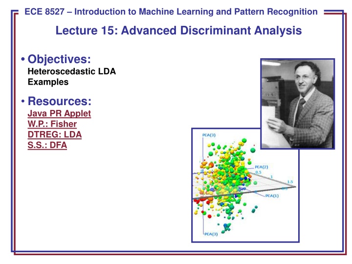
Heteroscedastic Linear Discriminant Analysis (HLDA) Heteroscedastic: when random variables have different variances. When might we observe heteroscedasticity? Suppose 100 students enroll in a typing class some of which have typing experience and some of which do not. After the first class there would be a great deal of dispersion in the number of typing mistakes. After the final class the dispersion would be smaller. The error variance is non-constant it decreases as time increases. An example is shown to the right. The two classes have nearly the same mean, but different variances, and the variances differ in one direction. LDA would project these classes onto a line that does not achieve maximal separation. HLDA seeks a transform that will account for the unequal variances. HLDA is typically useful when classes have significant overlap. ECE 8527: Lecture 15, Slide 1

Partitioning Our Parameter Vector Let W be partitioned into the first p columns corresponding to the dimensions we retain, and the remaining d-p columns corresponding to the dimensions we discard. Then the dimensionality reduction problem can be viewed in two steps: A non-singular transform is applied to x to transform the features, and A dimensionality reduction is performed where reduce the output of this linear transformation, y, to a reduced dimension vector, yp. Let us partition the mean and variances as follows: j,1 p j 0 p j ( 0 ) pxp j, p = = = j j ( ( ) ) d d p p + 0, p 1 ( ) x d p 0, d p j where is common to all terms and are different for each class. ECE 8527: Lecture 15, Slide 2

Density and Likelihood Functions The density function of a data point under the model, assuming a Gaussian model (as we did with PCA and LDA), is given by: T ( ) ( ) x x ( ) ( ) i g i i g i ( ) g i ( ) x = 2 P e i ( ) n 2 ( ) g i where is an indicator function for the class assignment for each data point. (This simply represents the density function for the transformed data.) (i ) g The log likelihood function is given by: ( , , log = j i j F x L ) 1 N T n ( + + i {( 1 = ) ) log(( 2 ) )} log x x ( ) ( ) i g i i g i ( ) ( ) g i g i 2 Differentiating the likelihood with respect to the unknown means and variances gives: ~ ~ j j X = ~ X ~ p T n = 0 p j ~ ~ 1 1 N ~ C ~ C p j T p p n T n = ( j = ( ) ) p p p n p N j ECE 8527: Lecture 15, Slide 3

Optimal Solution Substituting the optimal values into the likelihood equation, and then maximizing with respect to gives: N c p n p n F = = N j T T n + argmax { log log log } C C N p n p 2 2 1 j These equations do not have a closed-form solution. For the general case, we must solve them iteratively using a gradient descent algorithm and a two-step process in which we estimate means and variances from and then estimate the optimal value of from the means and variances. Simplifications exist for diagonal and equal covariances, but the benefits of the algorithm seem to diminish in these cases. To classify data, one must compute the log-likelihood distance from each class and then assign the class based on the maximum likelihood. Let s work some examples (class-dependent PCA, LDA and HLDA). HLDA training is significantly more expensive than PCA or LDA, but classification is of the same complexity as PCA and LDA because this is still essentially a linear transformation plus a Mahalanobis distance computation. ECE 8527: Lecture 15, Slide 4

Summary HLDA is used when random variables have different variances. There are many other forms of component analysis including neural network- based approaches (e.g., nonlinear PCA, learning vector quantization LVQ), kernel-based approaches that use data-driven kernels, probabilistic ICA, and support vector machines. ECE 8527: Lecture 15, Slide 5