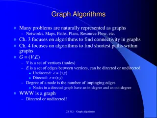
Advanced Graph Algorithms for Shortest Path Finding
Explore advanced graph algorithms such as Bellman-Ford and Floyd-Warshall for finding shortest paths in graphs with negative edges and detecting negative weight cycles. Understand the working mechanism, importance of optimum substructure, and dynamic programming concepts for efficient path determination.

Download Presentation

Please find below an Image/Link to download the presentation.
The content on the website is provided AS IS for your information and personal use only. It may not be sold, licensed, or shared on other websites without obtaining consent from the author. If you encounter any issues during the download, it is possible that the publisher has removed the file from their server.
You are allowed to download the files provided on this website for personal or commercial use, subject to the condition that they are used lawfully. All files are the property of their respective owners.
The content on the website is provided AS IS for your information and personal use only. It may not be sold, licensed, or shared on other websites without obtaining consent from the author.
E N D
Presentation Transcript
*Bellman-Ford: single-source shortest distance *O(VE) for graphs with negative edges *Detects negative weight cycles *Floyd-Warshall: All pairs shortest distance *O(V^3) *Overview
Weight function w(a,b): weight of the direct path from a to b Each vertex v has attributes: d: current minimum distance from start to v Previous: the vertex in the current shortest path from start to v just before v Relax(u,v,w): if v.d>u.d+w(u,v) v.d=u.d+w(u,v) v.previous=u *Bellman-Ford
*Bellman-Ford(G,w,s) Set all v.d= and s.d=0 Set all v.previous=null For i=1 to |G.V|-1 For each edge (u,v) in G.E Relax(u,v,w) *Bellman Ford
*Why does it work? *The shortest path from s to v contains at most |G.V|-1 edges. Consider a shortest path p <s,v1,v2,v3,v4 ,vn>. For each iteration of the first for loop we add a vertex to this shortest path. E.g.: v1.previous=S. The shortest path from S to v1 is saved as v1.d. We now add v2 (because it is reachable from v1) and v2.previous=v1. This is never overwritten because v1 is indeed in the shortest path from s to v2 (because otherwise p would not be the shortest path: otherwise replace v1 by vx and we have created a shorter path). By induction it follows that after |G.V|-1 iterations we have considered all shortest paths with |G.V|-1 edges.
For each edge (u,v) in G.E if v.d>u.d+w(u,v) return False Return True Proof: Returns true correctly because: v.d=s(s,d)<=s(s,u)+w(u,v)=u.d+w(u,v) Suppose <v0,v2, .,vn> is a negative edge cycle accessible from s where v0=vn: Assume returns true. Then vi.d<=v(i-1).d+w(v(i-1),vi) for 1 to n. Sum from i=1 to n-> 0<=w(v(i-1),vi), which contradicts: sum_1_n(w(vi-1,vi))<0 *Negative Cycle Check
*Shortest-Path algorithm has optimum substructure: *Consider shortest path v1->v2 with intermediate vertex vi. Then v1-> ->vi must be the shortest path from v1->vi and vi- > ->v2 must be the shortest path from vi->v2. Dynamic programming: *We don t know which intermediate vertex to choose. We want all pair shortest-paths. *Floyd-Warshall
*Define A[a][b][k] to be the length of the shortest path from a to b with possible intermediate vertices 1,2,3, k. *Set A[a][b][0] to the weight of the edge connecting a to b. *Recursive relation: A[a][b][k+1]= *Min(A[a][k+1][k]+A[K+1][b][k]), A[a][b][k]) *Because we only need a single level of k we can use O(V^2) memory if desirable. *Floyd-Warshall
*Code: *Set A[a][b][0]=w(a,b) *For k=1 to |V| For a=1 to |V| for b=1 to |V| A[a][b][k]=min(A[a][b][k-1],A[a][k][k-1]+A[k][b][k-1]) O(V^3) time


: weight of the direct path from a to")
")

 in G.E")
 in G.E")