Advanced Methods in Bayesian Belief Networks Classification
Bayesian belief networks, also known as Bayesian networks, are graphical models that allow class conditional independencies between subsets of variables. These networks represent dependencies among variables and provide a specification of joint probability distribution. Learn about classification methods using Bayesian belief networks, backpropagation, support vector machines, and frequent patterns. Explore scenarios for training Bayesian networks and understand the concepts behind them.

Download Presentation

Please find below an Image/Link to download the presentation.
The content on the website is provided AS IS for your information and personal use only. It may not be sold, licensed, or shared on other websites without obtaining consent from the author.If you encounter any issues during the download, it is possible that the publisher has removed the file from their server.
You are allowed to download the files provided on this website for personal or commercial use, subject to the condition that they are used lawfully. All files are the property of their respective owners.
The content on the website is provided AS IS for your information and personal use only. It may not be sold, licensed, or shared on other websites without obtaining consent from the author.
E N D
Presentation Transcript
Data Mining: Concepts and Techniques Chapter 9 1
Chapter 9. Classification: Advanced Methods Bayesian Belief Networks Classification by Backpropagation Support Vector Machines Classification by Using Frequent Patterns Lazy Learners (or Learning from Your Neighbors) Other Classification Methods Additional Topics Regarding Classification Summary 2
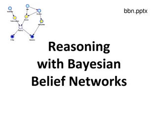
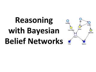
Bayesian Belief Networks Bayesian belief networks (also known as Bayesian networks, probabilistic networks): allow class conditional independencies between subsets of variables A (directed acyclic) graphical model of causal relationships Represents dependency among the variables Gives a specification of joint probability distribution Nodes: random variables Links: dependency X and Y are the parents of Z, and Y is the parent of P No dependency between Z and P Has no loops/cycles Y X Z P 3
Bayesian Belief Network: An Example CPT: Conditional Probability Table for variable LungCancer: Family History (FH) Smoker (S) (FH, S) (FH, ~S) (~FH, S) (~FH, ~S) LC 0.8 0.7 0.5 0.1 LungCancer (LC) ~LC 0.2 0.5 0.3 0.9 Emphysema shows the conditional probability for each possible combination of its parents Derivation of the probability of a particular combination of values of X, from CPT: PositiveXRay Dyspnea n Bayesian Belief Network = = ( ,..., ) ( | )) P x x P ( Parents Y xi i 1 n 1 i 4
Training Bayesian Networks: Several Scenarios Scenario 1: Given both the network structure and all variables observable: compute only the CPT entries Scenario 2: Network structure known, some variables hidden: gradient descent (greedy hill-climbing) method, i.e., search for a solution along the steepest descent of a criterion function Weights are initialized to random probability values At each iteration, it moves towards what appears to be the best solution at the moment, w.o. backtracking Weights are updated at each iteration & converge to local optimum Scenario 3: Network structure unknown, all variables observable: search through the model space to reconstruct network topology Scenario 4: Unknown structure, all hidden variables: No good algorithms known for this purpose D. Heckerman. A Tutorial on Learning with Bayesian Networks. In Learning in Graphical Models, M. Jordan, ed.. MIT Press, 1999. 5
Chapter 9. Classification: Advanced Methods Bayesian Belief Networks Classification by Backpropagation Support Vector Machines Classification by Using Frequent Patterns Lazy Learners (or Learning from Your Neighbors) Other Classification Methods Additional Topics Regarding Classification Summary 6
Classification by Backpropagation Backpropagation: A neural network learning algorithm Started by psychologists and neurobiologists to develop and test computational analogues of neurons A neural network: A set of connected input/output units where each connection has a weight associated with it During the learning phase, the network learns by adjusting the weights so as to be able to predict the correct class label of the input tuples Also referred to as connectionist learning due to the connections between units 7
Neural Network as a Classifier Weakness Long training time Require a number of parameters typically best determined empirically, e.g., the network topology or structure. Poor interpretability: Difficult to interpret the symbolic meaning behind the learned weights and of hidden units in the network Strength High tolerance to noisy data Ability to classify untrained patterns Well-suited for continuous-valued inputs and outputs Successful on an array of real-world data, e.g., hand-written letters Algorithms are inherently parallel Techniques have recently been developed for the extraction of rules from trained neural networks 8
A Multi-Layer Feed-Forward Neural Network Output vector ) 1 + = + ( ( ) ( ) k k k y ( ) w w y x j j i i ij Output layer Hidden layer wij Input layer Input vector: X 9
How A Multi-Layer Neural Network Works The inputs to the network correspond to the attributes measured for each training tuple Inputs are fed simultaneously into the units making up the input layer They are then weighted and fed simultaneously to a hidden layer The number of hidden layers is arbitrary, although usually only one The weighted outputs of the last hidden layer are input to units making up the output layer, which emits the network's prediction The network is feed-forward: None of the weights cycles back to an input unit or to an output unit of a previous layer From a statistical point of view, networks perform nonlinear regression: Given enough hidden units and enough training samples, they can closely approximate any function 10
Defining a Network Topology Decide the network topology: Specify # of units in the input layer, # of hidden layers (if > 1), # of units in each hidden layer, and # of units in the output layer Normalize the input values for each attribute measured in the training tuples to [0.0 1.0] One input unit per domain value, each initialized to 0 Output, if for classification and more than two classes, one output unit per class is used Once a network has been trained and its accuracy is unacceptable, repeat the training process with a different network topology or a different set of initial weights 11
Backpropagation Iteratively process a set of training tuples & compare the network's prediction with the actual known target value For each training tuple, the weights are modified to minimize the mean squared error between the network's prediction and the actual target value Modifications are made in the backwards direction: from the output layer, through each hidden layer down to the first hidden layer, hence backpropagation Steps Initialize weights to small random numbers, associated with biases Propagate the inputs forward (by applying activation function) Backpropagate the error (by updating weights and biases) Terminating condition (when error is very small, etc.) 12
Neuron: A Hidden/Output Layer Unit bias k x0 w0 x1 w1 f output y xn wn Example For n = = y sign( ) w ix i k Input vector x weight vector w weighted sum Activation function i 0 An n-dimensional input vector x is mapped into variable y by means of the scalar product and a nonlinear function mapping The inputs to unit are outputs from the previous layer. They are multiplied by their corresponding weights to form a weighted sum, which is added to the bias associated with unit. Then a nonlinear activation function is applied to it. 13
Efficiency and Interpretability Efficiency of backpropagation: Each epoch (one iteration through the training set) takes O(|D| * w), with |D| tuples and w weights, but # of epochs can be exponential to n, the number of inputs, in worst case For easier comprehension: Rule extraction by network pruning Simplify the network structure by removing weighted links that have the least effect on the trained network Then perform link, unit, or activation value clustering The set of input and activation values are studied to derive rules describing the relationship between the input and hidden unit layers Sensitivity analysis: assess the impact that a given input variable has on a network output. The knowledge gained from this analysis can be represented in rules 14
Chapter 9. Classification: Advanced Methods Bayesian Belief Networks Classification by Backpropagation Support Vector Machines Classification by Using Frequent Patterns Lazy Learners (or Learning from Your Neighbors) Other Classification Methods Additional Topics Regarding Classification Summary 15
Classification: A Mathematical Mapping Classification: predicts categorical class labels E.g., Personal homepage classification xi = (x1, x2, x3, ), yi = +1 or 1 x1: # of word homepage x2: # of word welcome Mathematically, x X = n, y Y = {+1, 1}, We want to derive a function f: X Y Linear Classification Binary Classification problem Data above the red line belongs to class x Data below red line belongs to class o Examples: SVM, Perceptron, Probabilistic Classifiers x x x x x x x o x x x o o ooo o o o o o o o 16
Discriminative Classifiers Advantages Prediction accuracy is generally high As compared to Bayesian methods in general Robust, works when training examples contain errors Fast evaluation of the learned target function Bayesian networks are normally slow Criticism Long training time Difficult to understand the learned function (weights) Bayesian networks can be used easily for pattern discovery Not easy to incorporate domain knowledge Easy in the form of priors on the data or distributions 17
SVMSupport Vector Machines A relatively new classification method for both linear and nonlinear data It uses a nonlinear mapping to transform the original training data into a higher dimension With the new dimension, it searches for the linear optimal separating hyperplane(i.e., decision boundary ) With an appropriate nonlinear mapping to a sufficiently high dimension, data from two classes can always be separated by a hyperplane SVM finds this hyperplane using support vectors( essential training tuples) and margins (defined by the support vectors) 18
SVMHistory and Applications Vapnik and colleagues (1992) groundwork from Vapnik & Chervonenkis statistical learning theory in 1960s Features: training can be slow but accuracy is high owing to their ability to model complex nonlinear decision boundaries (margin maximization) Used for: classification and numeric prediction Applications: handwritten digit recognition, object recognition, speaker identification, benchmarking time-series prediction tests 19
SVMGeneral Philosophy Small Margin Large Margin Support Vectors 20
SVMMargins and Support Vectors February 16, 2025 Data Mining: Concepts and Techniques 21
SVMWhen Data Is Linearly Separable m Let data D be (X1, y1), , (X|D|, y|D|), where Xi is the set of training tuples associated with the class labels yi There are infinite lines (hyperplanes) separating the two classes but we want to find the best one (the one that minimizes classification error on unseen data) SVM searches for the hyperplane with the largest margin, i.e., maximum marginal hyperplane (MMH) 22
SVMLinearly Separable A separating hyperplane can be written as W X + b = 0 where W={w1, w2, , wn} is a weight vector and b a scalar (bias) For 2-D it can be written as w0 + w1 x1 + w2 x2 = 0 The hyperplane defining the sides of the margin: H1: w0 + w1 x1 + w2 x2 1 for yi = +1, and H2: w0 + w1 x1 + w2 x2 1 for yi = 1 Any training tuples that fall on hyperplanes H1 or H2 (i.e., the sides defining the margin) are support vectors This becomes a constrained (convex) quadratic optimization problem: Quadratic objective function and linear constraints Quadratic Programming (QP) Lagrangian multipliers 23
Why Is SVM Effective on High Dimensional Data? The complexity of trained classifier is characterized by the # of support vectors rather than the dimensionality of the data The support vectors are the essential or critical training examples they lie closest to the decision boundary (MMH) If all other training examples are removed and the training is repeated, the same separating hyperplane would be found The number of support vectors found can be used to compute an (upper) bound on the expected error rate of the SVM classifier, which is independent of the data dimensionality Thus, an SVM with a small number of support vectors can have good generalization, even when the dimensionality of the data is high 24
A2 SVM Linearly Inseparable Transform the original input data into a higher dimensional space A1 Search for a linear separating hyperplane in the new space 25
SVM: Different Kernel functions Instead of computing the dot product on the transformed data, it is math. equivalent to applying a kernel function K(Xi, Xj) to the original data, i.e., K(Xi, Xj) = (Xi) (Xj) Typical Kernel Functions SVM can also be used for classifying multiple (> 2) classes and for regression analysis (with additional parameters) 26
Scaling SVM by Hierarchical Micro-Clustering SVM is not scalable to the number of data objects in terms of training time and memory usage H. Yu, J. Yang, and J. Han, Classifying Large Data Sets Using SVM with Hierarchical Clusters , KDD'03) CB-SVM (Clustering-Based SVM) Given limited amount of system resources (e.g., memory), maximize the SVM performance in terms of accuracy and the training speed Use micro-clustering to effectively reduce the number of points to be considered At deriving support vectors, de-cluster micro-clusters near candidate vector to ensure high classification accuracy 27
CF-Tree: Hierarchical Micro-cluster Read the data set once, construct a statistical summary of the data (i.e., hierarchical clusters) given a limited amount of memory Micro-clustering: Hierarchical indexing structure provide finer samples closer to the boundary and coarser samples farther from the boundary 28
Selective Declustering: Ensure High Accuracy CF tree is a suitable base structure for selective declustering De-cluster only the cluster Ei such that Di Ri < Ds, where Di is the distance from the boundary to the center point of Ei and Ri is the radius of Ei Decluster only the cluster whose subclusters have possibilities to be the support cluster of the boundary Support cluster : The cluster whose centroid is a support vector 29
CB-SVM Algorithm: Outline Construct two CF-trees from positive and negative data sets independently Need one scan of the data set Train an SVM from the centroids of the root entries De-cluster the entries near the boundary into the next level The children entries de-clustered from the parent entries are accumulated into the training set with the non- declustered parent entries Train an SVM again from the centroids of the entries in the training set Repeat until nothing is accumulated 30
Accuracy and Scalability on Synthetic Dataset Experiments on large synthetic data sets shows better accuracy than random sampling approaches and far more scalable than the original SVM algorithm 31
SVM vs. Neural Network SVM Neural Network Nondeterministic algorithm Generalizes well but doesn t have strong mathematical foundation Can easily be learned in incremental fashion To learn complex functions use multilayer perceptron (nontrivial) Deterministic algorithm Nice generalization properties Hard to learn learned in batch mode using quadratic programming techniques Using kernels can learn very complex functions 32
Chapter 9. Classification: Advanced Methods Bayesian Belief Networks Classification by Backpropagation Support Vector Machines Classification by Using Frequent Patterns Lazy Learners (or Learning from Your Neighbors) Other Classification Methods Additional Topics Regarding Classification Summary 33
Associative Classification Associative classification: Major steps Mine data to find strong associations between frequent patterns (conjunctions of attribute-value pairs) and class labels Association rules are generated in the form of P1 ^ p2 ^ pl Aclass= C (conf, sup) Organize the rules to form a rule-based classifier Why effective? It explores highly confident associations among multiple attributes and may overcome some constraints introduced by decision-tree induction, which considers only one attribute at a time Associative classification has been found to be often more accurate than some traditional classification methods, such as C4.5 34
Typical Associative Classification Methods CBA(Classification Based on Associations: Liu, Hsu & Ma, KDD 98) Mine possible association rules in the form of Cond-set (a set of attribute-value pairs) class label Build classifier: Organize rules according to decreasing precedence based on confidence and then support CMAR (Classification based on Multiple Association Rules: Li, Han, Pei, ICDM 01) Classification: Statistical analysis on multiple rules CPAR(Classification based on Predictive Association Rules: Yin & Han, SDM 03) Generation of predictive rules (FOIL-like analysis) but allow covered rules to retain with reduced weight Prediction using best k rules High efficiency, accuracy similar to CMAR 35
Frequent Pattern-Based Classification H. Cheng, X. Yan, J. Han, and C.-W. Hsu, Discriminative Frequent Pattern Analysis for Effective Classification , ICDE'07 Accuracy issue Increase the discriminative power Increase the expressive power of the feature space Scalability issue It is computationally infeasible to generate all feature combinations and filter them with an information gain threshold Efficient method (DDPMine: FPtree pruning): H. Cheng, X. Yan, J. Han, and P. S. Yu, "Direct Discriminative Pattern Mining for Effective Classification", ICDE'08 36
Frequent Pattern vs. Single Feature The discriminative power of some frequent patterns is higher than that of single features. (a) Austral (b) Cleve (c) Sonar Fig. 1. Information Gain vs. Pattern Length 37
Empirical Results 1 InfoGain IG_UpperBnd 0.9 0.8 0.7 Information Gain 0.6 0.5 0.4 0.3 0.2 0.1 0 0 100 200 300 400 500 600 700 Support (b) Breast (c) Sonar (a) Austral Fig. 2. Information Gain vs. Pattern Frequency 38
Feature Selection Given a set of frequent patterns, both non-discriminative and redundant patterns exist, which can cause overfitting We want to single out the discriminative patterns and remove redundant ones The notion of Maximal Marginal Relevance (MMR) is borrowed A document has high marginal relevance if it is both relevant to the query and contains minimal marginal similarity to previously selected documents 39
DDPMine: Branch-and-Bound Search child b sup( ) sup( ) parent sup( ) sup( ) a a b a: constant, a parent node Association between information gain and frequency b: variable, a descendent 40
DDPMine Efficiency: Runtime PatClass Harmony PatClass: ICDE 07 Pattern Classification Alg. DDPMine 41
Chapter 9. Classification: Advanced Methods Bayesian Belief Networks Classification by Backpropagation Support Vector Machines Classification by Using Frequent Patterns Lazy Learners (or Learning from Your Neighbors) Other Classification Methods Additional Topics Regarding Classification Summary 42
Lazy vs. Eager Learning Lazy vs. eager learning Lazy learning (e.g., instance-based learning): Simply stores training data (or only minor processing) and waits until it is given a test tuple Eager learning (the above discussed methods): Given a set of training tuples, constructs a classification model before receiving new (e.g., test) data to classify Lazy: less time in training but more time in predicting Accuracy Lazy method effectively uses a richer hypothesis space since it uses many local linear functions to form an implicit global approximation to the target function Eager: must commit to a single hypothesis that covers the entire instance space 43
Lazy Learner: Instance-Based Methods Instance-based learning: Store training examples and delay the processing ( lazy evaluation ) until a new instance must be classified Typical approaches k-nearest neighbor approach Instances represented as points in a Euclidean space. Locally weighted regression Constructs local approximation Case-based reasoning Uses symbolic representations and knowledge-based inference 44
The k-Nearest Neighbor Algorithm All instances correspond to points in the n-D space The nearest neighbor are defined in terms of Euclidean distance, dist(X1, X2) Target function could be discrete- or real- valued For discrete-valued, k-NN returns the most common value among the k training examples nearest toxq Vonoroi diagram: the decision surface induced by 1-NN for a typical set of training examples . _ _ _ _ . + . + . . _ + xq . _ + 45
Discussion on the k-NN Algorithm k-NN for real-valued prediction for a given unknown tuple Returns the mean values of the k nearest neighbors Distance-weighted nearest neighbor algorithm Weight the contribution of each of the k neighbors according to their distance to the query xq Give greater weight to closer neighbors Robust to noisy data by averaging k-nearest neighbors Curse of dimensionality: distance between neighbors could be dominated by irrelevant attributes To overcome it, axes stretch or elimination of the least relevant attributes 1 w 2 ) ix ( , d x q 46
Case-Based Reasoning (CBR) CBR: Uses a database of problem solutions to solve new problems Store symbolic description (tuples or cases) not points in a Euclidean space Applications: Customer-service (product-related diagnosis), legal ruling Methodology Instances represented by rich symbolic descriptions (e.g., function graphs) Search for similar cases, multiple retrieved cases may be combined Tight coupling between case retrieval, knowledge-based reasoning, and problem solving Challenges Find a good similarity metric Indexing based on syntactic similarity measure, and when failure, backtracking, and adapting to additional cases 47
Chapter 9. Classification: Advanced Methods Bayesian Belief Networks Classification by Backpropagation Support Vector Machines Classification by Using Frequent Patterns Lazy Learners (or Learning from Your Neighbors) Other Classification Methods Additional Topics Regarding Classification Summary 48
Genetic Algorithms (GA) Genetic Algorithm: based on an analogy to biological evolution An initial population is created consisting of randomly generated rules Each rule is represented by a string of bits E.g., if A1 and A2 then C2 can be encoded as 100 If an attribute has k > 2 values, k bits can be used Based on the notion of survival of the fittest, a new population is formed to consist of the fittest rules and their offspring The fitness of a rule is represented by its classification accuracy on a set of training examples Offspring are generated by crossover and mutation The process continues until a population P evolves when each rule in P satisfies a prespecified threshold Slow but easily parallelizable 49
Rough Set Approach Rough sets are used to approximately or roughly define equivalent classes A rough set for a given class C is approximated by two sets: a lower approximation (certain to be in C) and an upper approximation (cannot be described as not belonging to C) Finding the minimal subsets (reducts) of attributes for feature reduction is NP-hard but a discernibility matrix (which stores the differences between attribute values for each pair of data tuples) is used to reduce the computation intensity 50


")

")