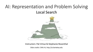
Explore the principles and applications of local search algorithms in solving complex problems with large search spaces, such as the N-queens problem. Learn about hill-climbing search, simulated annealing, genetic algorithms, and more. Dive into practical methods for optimizing solutions efficiently, even in the absence of complete information about the goal state.
Please find below an Image/Link to download the presentation.
The content on the website is provided AS IS for your information and personal use only. It may not be sold, licensed, or shared on other websites without obtaining consent from the author. If you encounter any issues during the download, it is possible that the publisher has removed the file from their server.
You are allowed to download the files provided on this website for personal or commercial use, subject to the condition that they are used lawfully. All files are the property of their respective owners.
The content on the website is provided AS IS for your information and personal use only. It may not be sold, licensed, or shared on other websites without obtaining consent from the author.
E N D
Presentation Transcript
CS 4700: Foundations of Artificial Intelligence Bart Selman selman@cs.cornell.edu Local Search Readings R&N: Chapter 4:1 and 6:4 1 Bart Selman CS4700
So far: methods that systematically explore the search space, possibly using principled pruning (e.g., A*) Current best such algorithm can handle search spaces of up to 10100 states / around 500 binary variables ( ballpark number only!) What if we have much larger search spaces? Search spaces for some real-world problems may be much larger e.g. 1030,000states as in certain reasoning and planning tasks. A completely different kind of method is called for --- non-systematic: Local search (sometimes called: Iterative Improvement Methods) 2 Bart Selman CS4700
Intro example: N-queens Problem: Place N queens on an NxN chess board so that no queen attacks another. Example solution for N = 8. How hard is it to find such solutions? What if N gets larger? Can be formulated as a search problem. Start with empty board. [Ops? How many?] Operators: place queen on location (i,j). [N^2. Goal?] Goal state: N queens on board. No-one attacks another. N=8, branching 64. Solution at what depth? N. Search: (N^2)^N Informed search? Ideas for a heuristic? N-Queens demo! Issues: (1) We don t know much about the goal state. That s what we are looking for! (2) Also, we don t care about path to solution! What algorithm would you write to solve this? 3 Bart Selman CS4700
Local Search: General Principle Key idea (surprisingly simple): 1) Select (random) initial state (initial guess at solution) e.g. guess random placement of N queens 2) Make local modification to improve current state e.g. move queen under attack to less attacked square 3) Repeat Step 2 until goal state found (or out of time) cycle can be done billions of times Unsolvable if out of time? Not necessarily! Method is incomplete. Requirements: generate an initial (often random; probably-not-optimal or even valid) guess evaluate quality of guess move to other state (well-defined neighborhood function) . . . and do these operations quickly . . . and don't save paths followed 4 Bart Selman CS4700
Local Search 1) 2) 3) 4) 5) Hill-climbing search or greedy local search Simulated annealing Local beam search (not covered) Genetic algorithms (related: genetic programming) Tabu search (not covered) 5 Bart Selman CS4700
Hill-climbing search Like climbing Everest in thick fog with amnesia Keep trying to move to a better neighbor , using some quantity to optimize. Note: (1) successor normally called neighbor. (2) minimization, isomorphic. (3) stops when no improvement but often better to just keep going , especially if improvement = 0 6 Bart Selman CS4700
4-Queens States: 4 queens in 4 columns (256 states) Neighborhood Operators: move queen in column Evaluation / Optimization function: h(n) = number of attacks / conflicts Goal test: no attacks, i.e., h(G) = 0 Initial state (guess). Local search: Because we only consider local changes to the state at each step. We generally make sure that series of local changes can reach all possible states. 7 Bart Selman CS4700
8-Queens 1 2 2 0 3 3 2 2 3 2 2 2 2 2 Representation: 8 integer variables giving positions of 8 queens in columns (e.g. <2, 5, 7, 4, 3, 8, 6, 1>) Section 6.4 R&N ( hill-climbing with min-conflict heuristics ) Pick initial complete assignment (at random) Repeat Pick a conflicted variable var (at random) Set the new value of var to minimize the number of conflicts If the new assignment is not conflicting then return it Inspired GSAT and Walksat (Min-conflicts heuristics) 8 Bart Selman CS4700
Local search with min-conflict heuristic works extremely well for N-queen problems. Can do millions and up in seconds. Similarly, for many other problems (planning, scheduling, circuit layout etc.) Why? Commonly given: Solns. are densely distributed in the O(nn) space; on average a solution is a few steps away from a randomly picked assignment. But, solutions still exponentially rare! In fact, density of solutions not very relevant. Even problems with a single solution can be easy for local search! It all depends on the structure of the search space and the guidance for the local moves provided by the optimization criterion. Remarks For N-queens, consider h(state) = k, if k queens are attacked. Does this still give a valid solution? Does it work as well? What happens if h(n) = 0 if no queen under attack; h(n) = 1 otherwise? Does this still give a valid solution? Does it work as well? What does search do? Blind local search! Provides no gradient in optimization criterion! 9 Bart Selman CS4700
Issues for hill-climbing search Problem: depending on initial state, can get stuck in local optimum (here maximum) How to overcome local optima and plateaus ? Random-restart hill climbing But, 1D figure is deceptive. True local optima are surprisingly rare in high-dimensional spaces! There often is an escape to a better state. 10 Bart Selman CS4700
Potential Issues with Hill Climbing / Greedy Local Search Local Optima: No neighbor is better, but not at global optimum. May have to move away from goal to find (best) solution. But again, true local optima are rare in many high-dimensional spaces. Plateaus: All neighbors look the same. 8-puzzle: perhaps no action will change # of tiles out of place. Soln. just keep moving around! (will often find some improving move eventually) Ridges: sequence of local maxima May not know global optimum: Am I done? 11 Bart Selman CS4700
Improvements to Greedy / Hill-climbing Search Issue: How to move more quickly to successively better plateaus? Avoid getting stuck / local maxima? Idea: Introduce noise: downhill (uphill) moves to escape from plateaus or local maxima (mimima) E.g., make a move that increases the number of attacking pairs. Noise strategies: 1. Simulated Annealing Kirkpatrick et al. 1982; Metropolis et al. 1953 2. Mixed Random Walk (Satisfiability) Selman, Kautz, and Cohen 1993 12 Bart Selman CS4700
Simulated Annealing Idea: Use conventional hill-climbing style techniques, but occasionally take a step in a direction other than that in which there is improvement (downhill moves; away from solution). As time passes, the probability that a down-hill step is taken is gradually reduced and the size of any down-hill step taken is decreased. 13 Bart Selman CS4700
Simulated annealing search (one of the most widely used optimization methods) What s the probability when: T inf? What s the probability when: T 0? What s the probability when: delta E = 0? (sideways / plateau move) Idea: escape local maxima by allowing some "bad" moves but gradually decrease frequency of such moves. their frequency Similar to hill climbing, but a random move instead of best move case of improvement, make the move Otherwise, choose the move with probability that decreases exponentially with the badness of the move. 14 Bart Selman CS4700
Notes Noise model based on statistical mechanics . . . introduced as analogue to physical process of growing crystals Convergence: 1. With exponential schedule, will provably converge to global optimum One can prove: If T decreases slowly enough, then simulated annealing search will find a global optimum with probability approaching 1 2. Few more precise convergence rate. (Recent work on rapidly mixing Markov chains. Surprisingly deep foundations.) Key aspect: downwards / sideways moves Expensive, but (if have enough time) can be best Thousands of papers; original paper one of most cited papers in CS! Many applications: VLSI layout, factory scheduling, protein folding. . . 15 Bart Selman CS4700
Simulated Annealing (SA) --- Foundations Superficially: SA is local search with some noise added. Noise starts high and is slowly decreased. True story is much more principled: SA is a general sampling strategy to sample from a combinatorial space according to a well-defined probability distribution. Sampling strategy models the way physical systems, such as gases, sample from their statistical equilibrium distributions. Order 10^23 particles. Studied in the field of statistical physics. We will give the core idea using an example. 16 Bart Selman CS4700
Example: 3D Hypercube space States Value f(s) s1 000 2 s2 001 4.25 s3 010 4 s4 011 3 s5 100 2.5 s6 101 4.5 s7 110 3 s8 111 3.5 Problem for greedy and hill climbing but not for SA! 110 111 100 101 010 011 000 Is there a local maximum? 001 N dimensional hypercube space. N =3. 2^3 = 8 states total. Goal: Optimize f(s), the value function. Maximum value 4.5 in s6. Use local search: Each state / node has N = 3 neighbors (out of 2^N total). Hop around to find 101 quickly. 17 Bart Selman CS4700
Of course, real interest in large N Spaces with 2^N states and each state with N neighbors. 9D hypercube; 512 states. How many steps to go from any state to any state? 7D hypercube; 128 states. Every node, connected to 7 others. Max distance between two nodes: 7. Practical reasoning problem: N = 1,000,000. 2^N = 10^300,000 18 Bart Selman CS4700
SA node sampling strategy Consider the following random walker in hypercube space: 1) Start at a random node S(the current node ). (How do we generate such a node?) 2) Select, at random, one of the N neighbors of S, call it S 3) (i.e., jump to node with better value) else with probability e^(f(S )-f(S))/T move to S , i.e., set S := S If (f(S ) f(S)) > 0, move to S , i.e. set S := S 4) Go back to 2) Note: Walker keeps going and going. Does not get stuck in any one node. 19 Bart Selman CS4700
Central Claim --- Equilibrium Distribution: After a while, we will find the walker in state S with probability Prob(S) = e^(f(S)/T) / Z where Z is a normalization constant (function of T) to make sure the probabilities over all states add up to 1. I.e., we will be in a state with a probability proportional to f(S) --- most likely in state with highest f(S). Why? Deep result in Markov Chain processes. Not obvious at all. Z is called the partition function and is given by Z = e^(f(s)/T) where the sum is over all 2^N states x. So, an exponential sum! Very hard to compute but we generally don t have to! 20 Bart Selman CS4700
For our example space Prob(s) = e^(f(s)/T) / Z States Value f(s) s1 000 2 s2 001 4.25 s3 010 4 s4 011 3 s5 100 2.5 s6 101 4.5 s7 110 3 s8 111 3.5 So, at T = 1.0, walker will spend roughly 29% of its time in the best state. T = 0.5, roughly 45% of its time in the best state. T = 0.25, roughly 65% of its time in the best state. And, remaining time mostly in s2 (2nd best)! T=0.5 Prob(s) 55 0.003 4915 0.27 2981 0.17 403 0.02 148 0.008 8103 0.45 403 0.02 1097 0.06 sum Z = 18,105 sum Z = 100,254,153 T=0.25 Prob(s) 2981 0.000 24,154,952 0.24 8,886,111 0.09 162,755 0.001 22,026 0.008 65,659,969 0.65 162,755 0.001 1,202,604 0.06 T=1.0 Prob(s) 7.4 0.02 70.1 0.23 54.6 0.18 20.1 0.07 12.2 0.04 90.0 0.29 20.1 0.07 33.1 0.11 sum Z = 307.9 21 Bart Selman CS4700
So, when T gets lowered, the probability distribution starts to concentrate on the maximum (and close to maximum) value states. The lower T, the stronger the effect! 2^N and 1/(2^N) because e^0 =1 in each row What about T high? What is Z and Prob(S)? At low T, we can just output the current state. It will quite likely be a maximum value (or close to it) state. In practice: Keep track of best state seen during the SA search. SA is an example of so-called Markov Chain Monte Carlo or MCMC sampling. It s very general technique to sample from complex probability distributions by making local moves only. For optimization, we chose a clever probability distribution that concentrates on the optimum states for low T. (Kirkpatrick et al. 1984) 22 Bart Selman CS4700
Some final notes on SA: 1) Claim Equilibrium Distribution needs proof. Not too difficult but takes a bit of background about Markov Chains. It s beautiful and useful theory. How long should we run at each T? Technically, till the process reaches the stationary distribution. Here s the catch: may take exponential time in the worst case. But in practice can be remarkably effective. How quickly should we cool down ? Various schedules in literature. To get (near-)optimum, you generally can run much shorter than needed for full stationary distribution. Keep track of best solution seen so far. A few formal convergence rate results exists, including some polytime results ( rapidly mixing Markov chains ). Many variations on basic SA exist, useful for different applications. 2) 3) 4) 5) 6) 7) 23 Bart Selman CS4700
What I didnt tell you Q. Why not just run at a low temperature right away? SA is guaranteed to converge to the equilibrium distribution Prob(s) = e^(f(s)/T) / Z However, this can take some time. Burn-in time of Markov chain. Idea of annealing: can reach equilibrium distribution more quickly by first starting at a higher T and going down slowly. Practical example: T = 100, take 100,000 flips. Then, T = .9 * 100 = 90, take 100,000 flips. Then, T = .9 * 90 = 81, take 100,000 flips. Etc. Q. How can you sample properly from an exponential space without the chain first visiting each state? Best answered with an example. Consider N binary variables, and starting from the all 0 state ( origin of hypercube ). How many flips are needed to reach a purely random point uniformly at random in the N dimensional hypercube? 24 Bart Selman CS4700
Genetic Algorithms Another class of iterative improvement algorithms A genetic algorithm maintains a population of candidate solutions for the problem at hand, and makes it evolve by iteratively applying a set of stochastic operators Inspired by the biological evolution process Uses concepts of Natural Selection and Genetic Inheritance (Darwin 1859) Originally developed by John Holland (1975) 26 Bart Selman CS4700
High-level Algorithm 1. 2. 3. Randomly generate an initial population Evaluate the fitness of members of population Select parents based on fitness, and reproduce to get the next generation (using crossover and mutations) Replace the old generation with the new generation Repeat step 2 though 4 till iteration N 4. 5. 27 Bart Selman CS4700
Stochastic Operators Cross-over decomposes two distinct solutions and then randomly mixes their parts to form novel solutions Mutation randomly perturbs a candidate solution 28 Bart Selman CS4700
A successor state is generated by combining two parent states Start with k randomly generated states (population) A state is represented as a string over a finite alphabet (often a string of 0s and 1s) Evaluation function (fitness function). Higher values for better states. Produce the next generation of states by selection, crossover, and mutation 29 Bart Selman CS4700
Genetic algorithms Operate on state representation. random mutation production of next generation Fitness function: number of non-attacking pairs of queens (min = 0, max = 8 7/2 = 28 the higher the better) crossover point randomly generated probability of a given pair selection proportional to the fitness (b) 24/(24+23+20+11) = 31% 30 Bart Selman CS4700
Genetic algorithms Any reason pieces from different solutions fit together? 31 Bart Selman CS4700
Lots of variants of genetic algorithms with different selection, crossover, and mutation rules. GAs have a wide application in optimization e.g., circuit layout and job shop scheduling Much work remains to be done to formally understand GAs and to identify the conditions under which they perform well. 32 Bart Selman CS4700
Demo of Genetic Programming (GP): The Evolutionary Walker GA: Current state: A program. Local change: Small change in program. Stick figure --- Three nodes: 1 body 2 feet Goal: Make it run as fast as possible! Evolve population of control programs. Basic physics model: gravity momentum etc. Programs computes actions to control: 1) angle 2) push off ground for each foot. Input for control programs (from physics module): Position and velocity for the three nodes. Discrete time 33 Bart Selman CS4700
Control programming language: Example: Basically, computes a real number to set angle (or push strength) for next time step. Body and feet will each evolve their own control program. 34 Bart Selman CS4700
Population of control programs is maintained and evolved. Fitness determined by measuring how far the walker gets in T time units (T fixed). Evolution through parent selection based on fitness. Followed by crossover (swap parts of control programs, i.e., arithmetic expression trees) and mutations (randomly generate new parts of control program). 35 Bart Selman CS4700
Can this work? How well? Would it be hard to program directly? Think about it Demo 36 Bart Selman CS4700
1) Surprisingly efficient search technique 2) Often the only feasible approach 3) Wide range of applications 4) Formal properties / guarantees still difficult to obtain 5) Intuitive explanation: Search spaces are too large for systematic search anyway. . . 6) Area will most likely continue to thrive 43 Bart Selman CS4700


 --- Foundations")


:")


(/(U(N 2))(Y(N 0))))(I(B")
(*(/(X(N 0))(I(B true)(Y(N 1))(-(Y(N 2))(R")
))))(+(Y(N 2))(R -1.6972810613722311)))(-(Y(N 2))(+(X(N")

 Surprisingly efficient search technique")