Advanced Topics in Expectation Maximization (EM) and Pattern Recognition
Discover a comprehensive exploration of Expectation Maximization (EM) including the Special Case of Jensen's Inequality, EM Theorem Proof, EM application in Hidden Markov Models, and the Expectation Maximization Algorithm. Understand the iterative optimization method of EM used in various probabilistic models to estimate unknown parameters and uncover hidden variables effectively.

Download Presentation

Please find below an Image/Link to download the presentation.
The content on the website is provided AS IS for your information and personal use only. It may not be sold, licensed, or shared on other websites without obtaining consent from the author. If you encounter any issues during the download, it is possible that the publisher has removed the file from their server.
You are allowed to download the files provided on this website for personal or commercial use, subject to the condition that they are used lawfully. All files are the property of their respective owners.
The content on the website is provided AS IS for your information and personal use only. It may not be sold, licensed, or shared on other websites without obtaining consent from the author.
E N D
Presentation Transcript
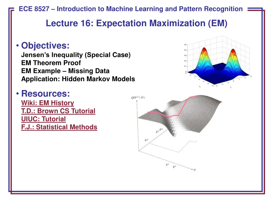
ECE 8443 Pattern Recognition ECE 8527 Introduction to Machine Learning and Pattern Recognition Lecture 16: Expectation Maximization (EM) Objectives: Jensen s Inequality (Special Case) EM Theorem Proof EM Example Missing Data Application: Hidden Markov Models Resources: Wiki: EM History T.D.: Brown CS Tutorial UIUC: Tutorial F.J.: Statistical Methods
Special Case of Jensens Inequality Lemma: If p(x) and q(x) are two discrete probability distributions, then: x x ( ) log ( ) ( ) log ( ) p x p x p x q x with equality if and only if p(x) = q(x) for all x. Proof: x q ( ) log ( ) ( ) log ( ) 0 p x p x p x q x x ( ) x ( ) log ( ) ( ) 0 p x p x x ( ) p x x ( ) log 0 p x ( ) q ( x ) q x x ( ) log 0 p x ( ) p x ( ) ( ) q x q x x x ( ) log ( )( ) 1 p x p x ( ) ( ) p x p x ( ) x x The last step follows using a bound for the natural logarithm: . ln 1 ECE 8527: Lecture 16, Slide 1
Special Case of Jensens Inequality Continuing in efforts to simplify: ( ) ( ) ( ) q x q x q x x x x x x x = = = ( ) log ( )( ) 1 ( ) ( ) ( ) ( ) . . 0 p x p x p x p x q x p x ( ) ( ) ( ) p x p x p x We note that since both of these functions are probability distributions, they must sum to 1.0. Therefore, the inequality holds. The general form of Jensen s inequality relates a convex function of an integral to the integral of the convex function and is used extensively in information theory. ECE 8527: Lecture 16, Slide 2
The Expectation Maximization Algorithm ECE 8527: Lecture 16, Slide 3
The Expectation Maximization Algorithm (Preview) ECE 8527: Lecture 16, Slide 4
The Expectation Maximization Algorithm (Cont.) ECE 8527: Lecture 16, Slide 5
The Expectation Maximization Algorithm ECE 8527: Lecture 16, Slide 6
Synopsis Expectation maximization (EM) is an approach that is used in many ways to find maximum likelihood estimates of parameters in probabilistic models. EM is an iterative optimization method to estimate some unknown parameters given measurement data. Used in a variety of contexts to estimate missing data or discover hidden variables. The intuition behind EM is an old one: alternate between estimating the unknowns and the hidden variables. This idea has been around for a long time. However, in 1977, Dempster, et al., proved convergence and explained the relationship to maximum likelihood estimation. EM alternates between performing an expectation (E) step, which computes an expectation of the likelihood by including the latent variables as if they were observed, and a maximization (M) step, which computes the maximum likelihood estimates of the parameters by maximizing the expected likelihood found on the E step. The parameters found on the M step are then used to begin another E step, and the process is repeated. This approach is the cornerstone of important algorithms such as hidden Markov modeling and discriminative training. It has also been applied to fields including human language technology and image processing. ECE 8527: Lecture 16, Slide 7
The EM Theorem Theorem: If then . ( ) ( ) ( ) P y t P y t P t t ( ) y t ( ( ) y t ) ( ) y ( ) y log log P P P ( ) y P Proof: Let y denote observable data. Let be the probability distribution of y under some model whose parameters are denoted by . ( ) y P Let be the corresponding distribution under a different setting . Our goal is to prove that y is more likely under than . Let t denote some hidden, or latent, parameters that are governed by the ( ) y t P values of . Because is a probability distribution that sums to 1, we can write: P log ( ) y t ( ) y t ( ) y ( ) y ( ) y ( ) y = t t log log log P P P P P Because we can exploit the dependence of y on t and using well-known properties of a conditional probability distribution. ECE 8527: Lecture 16, Slide 8
Proof Of The EM Theorem We can multiply each term by 1 : ( ( ) ) ( ( ) ) , , P t y P t y ( ) t ( ) t ( ) y ( ) y ( ) y ( ) y , = t t log log log log P P P y P P y P , , P t y P t y ( ( ) ( t , ) ( ( ) y t , ) , P t y P t y ( ) t ( ) y t P = t t log log P y P P t y P t y ( ) ( ) ( ) y t ( ) ( ) ( ) y t ( ) ) ( ( ) ) = t t log log P t y P y P t y ( ( ) t ) ( ( ) ) + t t log log , P t y P y P t y P t y ( ( ) ) ( ( ) ) t t log , log , P P t y P P t y where the inequality follows from our lemma. Explanation: What exactly have we shown? If the last quantity is greater than zero, then the new model will be better than the old model. This suggests a strategy for finding the new parameters, : choose them to make the last quantity positive! ECE 8527: Lecture 16, Slide 9
Discussion If we start with the parameter setting , and find a parameter setting for which our inequality holds, then the observed data, y, will be more probable under than . The name Expectation Maximization comes about because we take the ( ) y t P , ( ) y , P t expectation of with respect to the old distribution and then maximize the expectation as a function of the argument . Critical to the success of the algorithm is the choice of the proper intermediate variable, t, that will allow finding the maximum of the expectation ( ) ( ) ( ) y t P y t P t of . log Perhaps the most prominent use of the EM algorithm in pattern recognition is to derive the Baum-Welch reestimation equations for a hidden Markov model. Many other reestimation algorithms have been derived using this approach. ECE 8527: Lecture 16, Slide 10
Example: Estimating Missing Data ECE 8527: Lecture 16, Slide 11
Example: Estimating Missing Data ECE 8527: Lecture 16, Slide 12
Example: Estimating Missing Data ECE 8527: Lecture 16, Slide 13
Example: Estimating Missing Data ECE 8527: Lecture 16, Slide 14
Example: Estimating Missing Data ECE 8527: Lecture 16, Slide 15
Example: Gaussian Mixtures An excellent tutorial on Gaussian mixture estimation can be found at J. Bilmes, EM Estimation An interactive demo showing convergence of the estimate can be found at I. Dinov, Demonstration ECE 8527: Lecture 16, Slide 16
Summary Expectation Maximization (EM) Algorithm: a generalization of Maximum Likelihood Estimation (MLE) based on maximization of a posterior that data was generated by a model. EM is a special case of Jensen s inequality. Jensen s Inequality: describes a relationship between two probability distributions in terms of an entropy-like quantity. A key tool in proving that EM estimation converges. The EM Theorem: proved that estimation of a model s parameters using an iteration of EM increases the posterior probability that the data was generated by the model. Demonstrated an application of the EM Theorem to the problem of estimating missing data point. Explained how EM can be used to reestimate parameters in a pattern recognition system. ECE 8527: Lecture 16, Slide 17


")
")