Algorithms in the Real World: Cache-aware Sorting and Locality Improvement
Discussing cache-aware algorithms, B-trees, buffer trees, and the RAM model in real-world environments. Exploring memory hierarchy, I/O models, and the benefits of a 2-level hierarchy. Comparing performance improvements in various algorithms.

Download Presentation

Please find below an Image/Link to download the presentation.
The content on the website is provided AS IS for your information and personal use only. It may not be sold, licensed, or shared on other websites without obtaining consent from the author.If you encounter any issues during the download, it is possible that the publisher has removed the file from their server.
You are allowed to download the files provided on this website for personal or commercial use, subject to the condition that they are used lawfully. All files are the property of their respective owners.
The content on the website is provided AS IS for your information and personal use only. It may not be sold, licensed, or shared on other websites without obtaining consent from the author.
E N D
Presentation Transcript
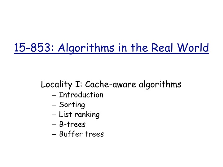
15-853: Algorithms in the Real World Locality I: Cache-aware algorithms Introduction Sorting List ranking B-trees Buffer trees
RAM Model Standard theoretical model for analyzing algorithms: Infinite memory size Uniform access cost Evaluate an algorithm by the number of instructions executed CPU RAM
Real Machine Example: Nehalem CPU L3 cache size: 24MB line size: 64B access time: 20ns Memory access time: 100ns Disc access time: ~4ms = 4x10⁶ns The cost of transferring data is important Design algorithms with locality in mind ~ 0.4ns / instruction 8 Registers L1 cache size: 64KB line size: 64B access time: 1.5ns L2 cache size: 256KB line size: 64B access time: 5ns Main Memory L3 CPU L1 Disc L2
I/O Model Abstracts a single level of the memory hierarchy Fast memory (cache) of size M Accessing fast memory is free, but moving data from slow memory is expensive Memory is grouped into size-Bblocks of contiguous data B Fast Memory Slow Memory CPU block M/B B Cost: the number of block transfers (or I/Os) from slow memory to fast memory.
Notation Clarification M: the number of objects that fit in memory, and B: the number of objects that fit in a block So for word-size (8 byte) objects,and memory size 1Mbyte, M = 128,000
Why a 2-Level Hierarchy? It s simpler than considering the multilevel hierarchy A single level may dominate the runtime of the application, so designing an algorithm for that level may be sufficient Considering a single level exposes the algorithmic difficulties generalizing to a multilevel is often straightforward We ll see cache-oblivious algorithms later as a way of designing for multi-level hierarchies
What Improvement Do We Get? Examples Adding all the elements in a size-N array (scanning) Sorting a size-N array Searching a size-N data set in a good data structure Problem RAM Algorithm Scanning (N) Sorting (N log2N) Searching (log2N) Permuting (N) For 8-byte words on example new Intel Processor B 8 in L2-cache, B 1000 on disc log2B 3 in L2-cache, log2B 10 on disc I/O Algorithm (N/B) ((N/B)logM/B(N/B)) (logBN) (min(N,sort(N))
Sorting Standard MergeSort algorithm: Split the array in half MergeSort each subarray Merge the sorted subarrays Number of computations is O(N logN) on an N-element array How does the standard algorithm behave in the I/O model?
Merging block B = 4 1 3 8 15 20 22 25 26 30 45 52 63 + 2 4 6 7 10 24 29 33 34 36 37 39 1 2 3 4 6 7 8 A size-N array occupies at most N/B +1 blocks Each block is loaded once during merge, assuming memory size M 3B
MergeSort Analysis Sorting in memory is free, so the base case is S(M) = (M/B) to load a size-M array S(N) = 2S(N/2) + (N/B) S(N) = ((N/B)(log2(N/M)+1)) N log2(N/M) N/2 2M M
I/O Efficient MergeSort Instead of doing a 2-way merge, do a (M/B)- way merge IOMergeSort: Split the array into (M/B) subarrays IOMergeSort each subarray Perform a (M/B)-way merge to combine the subarrays
k-Way Merge k Assuming M/B k+1, one block from each array fits in memory Therefore, only load each block once Total cost is thus (N/B)
IOMergeSort Analysis Sorting in memory is free, so the base case is S(M) = (M/B) to load a size-M array S(N) = (M/B) S(NB/M) + (N/B) S(N) = ((N/B)(logM/B(N/M)+1)) N logM/B(N/M) N/(M/B) M2/B M
MergeSort Comparison Traditional MergeSort costs ((N/B)log2(N/M)) I/Os on size-N array IOMergeSort is I/O efficient, costing only ((N/B)logM/B(N/M)) The new algorithm saves (log2(M/B)) fraction of I/Os. How significant is this savings? Consider L3 cache to main memory on Nehalem M = 1 Million, B = 8, N = 1 Billion 1 billion / 8 x 10 vs. 1 billion / 8 x 1 Not hard to calculate exact constants
List Ranking Given a linked list, calculate the rank of (number of elements before) each element 9 2 7 1 6 5 0 8 3 4 start Trivial algorithm is O(N) computation steps
List ranking in I/O model Assume list is stored in ~N/B blocks! May jump in memory a lot. Example: M/B = 3, B = 2, least-recently-used eviction 9 2 7 1 6 5 0 8 3 4 start In general, each pointer can result in a new block transfer, for O(N) I/Os
Why list ranking? Recovers locality in the list (can sort based on the ranking) 9 0 1 2 3 4 5 6 7 8 start Generalizes to trees via Euler tours Useful for various forest/tree algorithms like least common ancestors and tree contraction Also used in graph algorithms like minimum spanning tree and connected components
List ranking outline 1. Produce an independent set of (N) nodes (if a node is in the set, its successor is not) start 2. Bridge out independent set and solve weighted problem recursively 2 2 9 7 1 5 0 3 2 start 2 1
List ranking outline 1 9 7 1 5 0 3 1 start 3. Merge in bridged-out nodes 1 9 2 7 1 6 5 0 8 3 4 1 start
List ranking: 1) independent set Each node flips a coin {0,1} A node is in the independent set if it chooses 1 and its predecessor chooses 0 1 1 0 0 1 0 0 1 0 1 start Each node enters independent set with prob , so expected set size is (N).
List ranking: 1) independent set 1j 1a 0b 0c 1d 0e 0f 1g 0h 1i start Identifying independent-set nodes efficiently: Sort by successor address 1i 0b 1a 0c 0f 1d 0e 0h 1j 1g start After sort, requires O(scan(N ))=O(N/B) block transfers
List ranking: 2) bridging out Sort by successor address twice j a b c d e f g h i start i b a c f d e h j g start c a h d e i g b f j start
List ranking: 2) bridging out If middle node is in independent set, splice it out Gives a list of new pointers Sort back to original order and scan to integrate pointer updates a b c c f d x+y y a b c d e old e f j a b c d e update x
List ranking: 2) bridging out 1 j a b c d e f g h i start 2 Scans and sorts to compress and remove independent set nodes (homework) 2 1 2 b c e f h j 2 2 start
List ranking: 3) merge in 1 9 7 1 5 0 3 1 start Uses sorts and scans 1 9 2 7 1 6 5 0 8 3 4 1 start
List ranking analysis 1. Produce an independent set of (N) nodes (keep retrying until random set is good enough) 2. Bridge out and solve recursively 3. Merge-in bridged-out nodes All steps use a constant number of sorts and scans, so expected cost is O(sort(N)) = O((N/B) logM/B (N/B)) I/Os at this level of recursion Gives recurrence R(N) = R(N/c) + O(sort(N)) = O(sort(N))
B-Trees A B-tree is a type of search tree ((a,b)-tree) designed for good memory performance Common approach for storing searchable, ordered data, e.g., databases, filesystems. Operations Updates: Insert/Delete Queries Search: is the element there Successor/Predecessor: find the nearest key Range query: return all objects with keys within a range
B-tree/(2,3)-tree Objects stored in leaves Leaves all have same depth Root has at most B children Other internal nodes have between B/2 and B children B 18 35 6 10 25 43 50 1 2 4 10 12 15 18 21 25 28 35 37 50 51 53 6 8 43 45
B-tree search Compare search key against partitioning keys and move to proper child. Cost is O(height * node size) Search for 21 18 35 6 10 25 43 50 1 2 4 10 12 15 18 21 25 28 35 37 50 51 53 6 8 43 45
B-tree insert Search for where the key should go. If there s room, put it in Insert 23 18 35 6 10 25 43 50 1 2 4 10 12 15 18 21 23 25 28 35 37 50 51 53 6 8 43 45
B-tree insert Search for where the key should go. If there s no room, split the node Splits may propagate up tree Insert 24 18 35 6 10 25 23 25 43 50 1 2 4 10 12 15 18 21 23 25 28 35 37 50 51 53 6 8 23 24 43 45
B-tree inserts Splits divide the objects / child pointers as evenly as possible. If the root splits, add a new parent (this is when the height of the tree increases) Deletes are a bit more complicated, but similar if a node drops below B/2 children, it is merged or rebalanced with some neighbors.
B-tree analysis Search All nodes (except root) have at least (B) children height of tree is O(logBN) Each node fits in a block Total search cost is O(logBN) block transfers.
B-tree analysis Insert (and delete): Every split of a leaf results in an insert into a height-1 node. In general, a height-h split causes a height-(h+1) insert. There must be (B) inserts in a node before it splits again. An insert therefore pays for (1/B)h = O(1/B) splits, each costing O(1) block transfers. Searching and updating the keys along the root- to-leaf path dominates for O(logBN) block transfers
Sorting with a search tree? Consider the following RAM sort algorithm: 1. Build a balanced search tree 2. Repeatedly delete the minimum element from the tree Runtime is O(N logN) Does this same algorithm work in the I/O model? Just using a B-tree is O(N logBN) which is much worse than O((N/B) logM/B(N/B))
Buffer tree Somewhat like a B-tree: when nodes gain too many children, they split evenly, using a similar split method all leaves are at the same depth Unlike a B-tree: queries are not answered online (they are reported in batches) internal nodes have (M/B) children nodes have buffers of size (M)
Buffer-tree insert M Insert buffer buffer buffer M/B Start at root. Add item to end of buffer. If buffer is not full, done. Otherwise, partition the buffer and send elements down to children.
Buffer-tree insert M Insert buffer height O(logM/B(N/B)) buffer buffer M/B Analysis ideas: Inserting into a buffer costs O(1+k/B) for k elements inserted On overflow, partitioning costs O(M/B) to load entire buffer. Then M/B scans are performed, costing O(#Arrays + total size/B) = O(M/B + M/B) Flushing buffer downwards therefore costs O(M/B), moving (M) elements, for a cost of O(1/B) each per level An element may be moved down at each height, costing a total of O((1/B) height) = O((1/B)logM/B(N/B)) per element
I/O Priority Queue Supporting Insert and Extract-Min (no Decrease- Key here) Keep a buffer of (M) smallest elements in memory Use a buffer tree for remaining elements. While smallest-element buffer is too full, insert 1 (maximum) element into buffer tree If smallest-element buffer is empty, flush leftmost path in buffer tree and delete the leftmost leafs Total cost is O((N/B) logM/B(N/B)) for N ops. Yields optimal sort.
Buffer-tree variations To support deletions, updates, and other queries, insert records in the tree for each operation, associated with timestamps. As records with the same key collide, merge them as appropriate. Examples of applications: DAG shortest paths Circuit evaluation Computational geometry applications


 independent set")
 independent set")
 bridging out")
 bridging out")
 bridging out")
 merge in")


-tree")