Analysis of Local Search Heuristic for Facility Location Problem
Local search technique is explored for the facility location problem, involving operations like adding, dropping, and swapping facilities to improve cost. Primary and secondary facility concepts are discussed, along with neighborhood definitions and optimization strategies.

Uploaded on Apr 28, 2025 | 1 Views
Download Presentation

Please find below an Image/Link to download the presentation.
The content on the website is provided AS IS for your information and personal use only. It may not be sold, licensed, or shared on other websites without obtaining consent from the author.If you encounter any issues during the download, it is possible that the publisher has removed the file from their server.
You are allowed to download the files provided on this website for personal or commercial use, subject to the condition that they are used lawfully. All files are the property of their respective owners.
The content on the website is provided AS IS for your information and personal use only. It may not be sold, licensed, or shared on other websites without obtaining consent from the author.
E N D
Presentation Transcript
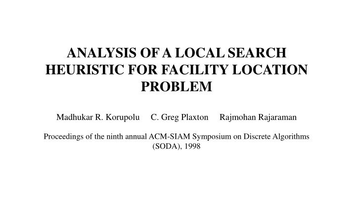
ANALYSIS OF A LOCAL SEARCH HEURISTIC FOR FACILITY LOCATION PROBLEM Madhukar R. Korupolu C. Greg Plaxton Rajmohan Rajaraman Proceedings of the ninth annual ACM-SIAM Symposium on Discrete Algorithms (SODA), 1998
LOCAL SEARCH TECHNIQUE 1. Choose a feasible solution S arbitrarily. 2. Apply a local search operation on S to obtain a new solution with improved cost. 3. Repeat step 2 until no more operations can be performed that improves the existing cost. 4. Output the current solution S as local optimal solution.
LOCAL SEARCH OPERATIONS 1. Adding a facility 2. Dropping a facility 3. Swapping a facility Assumption:- All the operations can be done in polynomial time.
Adding a facility A new facility which does not belong to the current solution is added to it. Reassignment of the clients is done. If there is an improvement in the total cost, the facility is added, else rejected.
Dropping a facility A facility is dropped from the current solution. The clients of the dropped facility are reassigned to the other facilities in the solution. If there is an improvement in the total cost, the facility is dropped, else not.
Swapping a facility A facility of the current solution is swapped with a new facility which does not belong to the current solution. Reassignment of the clients is done. If there is an improvement in the total cost, the facility is swapped, else not.
IMPORTANT TERMS 1. Primary Facility 2. Secondary Facility
PRIMARY FACILITY For each facility i* in the optimal solution, Neighborhood of i*, denoted as N(i*) is the set of i S such that i* is closest to i in optimal. A facility i N(i*) is said to be a primary facility if it is closest to i*. O i* C indicates closest edge S i i N(i*) Primary facility
SECONDARY FACILITY All the facilities in the current solution which are not tagged as primary facilities are secondary facilities. O i* C S i i N(i*) Associated Primary Facility Secondary Facility For a secondary facility i N(i*), i is said to be its associated primary facility if i is primary facility of i*.
ANALYSIS S:- Local Optimal solution O:- Global Optimal solution. gi = total service cost paid by clients of facility i S gi* = total service cost paid by clients of facility i O Sp = set of all primary facilities in S Ss = set of all secondary facilities in S S O = Since S is the local optimal solution, therefore, its cost cannot be improved further by performing any operation. Add operation is used to bound the service cost of S. Drop and Swap operation are used to bound the facility opening cost of S.
BOUNDING SERVICE COST Consider a facility o O added to S to give S . C(S ) C(S) = fo + go* go O + + + + + + + + + + + + C -- - - - - - - - - - - S Since S is locally optimum, fo + go* go 0 ==> go fo + go* After doing this for all the facilities of optimal and adding them, we get Cs(S) Cf(O) + Cs(O).
BOUNDING FACILITY COST OF SECONDARY FACILITIES USING DROP OPERATION Drop operation is performed on secondary facilities. Consider a secondary facility i being dropped from S to give a new solution S , i.e., S = S - i. All the clients of i are reassigned to its associated primary facility i in S. Difference in total cost of S and S is, C(S ) - C(S). Since S is locally optimum, => C(S ) C(S) 0 Consider all the clients j of i, which are now reassigned to i , therefore, C(S ) C(S) = j (cji cji) fi 0 fi j (cji cji) ..I
Let i N(i*). Then i also in N(i*) i i* O j C - + i i S cji cji + cii* + ci*i cji + 2cii* (since i is primary facility of i*) cji + 2ci i cji - cji 2(cji + cji ) (by triangle inequality) cji - cji 2(cji + cji*) (since j is assigned to i ) Adding this for all the clients of i Ss, we get j(cji - cji) 2(gi + gi*). Therefore eq I now becomes, fi 2(gi + gi*). Adding this for all secondary facilities i Ss leads to, Cf(Ss) i 2(gi + gi*) (by triangle inequality) (i*, and not i , is closest to i)
BOUNDING FACILITY COST OF SECONDARY FACILITIES USING SWAP OPERATION Swap operation is performed on primary facilities. Consider a primary facility i being swapped with its closest facility i* O to give a new solution S , i.e., S = S i + i*. All the clients of i are reassigned to i*. Difference in total cost of S and S is, C(S ) C(S). Since S is locally optimum, => C(S ) C(S) 0 Consider all the clients j of i, which are now reassigned to i*, therefore, C(S ) C(S) = j (cji cji) fi + fi* 0 fi fi* j (cji cji) ..I
i i* O j C - + i S cji* cji + cii* cji + cii cji* - cji (cji + cji ) (by triangle inequality) cji* - cji cji + cji*(since j is assigned to i ) Adding this for all the clients of i Sp, we get j(cji* - cji) gi+gi* Therefore eq I becomes, fi - fi* (gi + gi*). Adding this for all primary facilities i Sp leads to, Cf(Sp)- Cf(O) i (gi + gi*) (by triangle inequality) (since i* is closest to i)
BOUNDING TOTAL COST Adding results of drop and swap, we get Cf(S) Cf(O) + 2Cs(S) + 2Cs(O) Using the following bound on service cost from add operation, Cs(S) Cf(O) + Cs(O) we get, C(S) 4 Cf(O) + 5 Cs(O)


. Then i’ also in N(i*)")