Analysis of Sample Size Calculation Methods for Statistical Studies

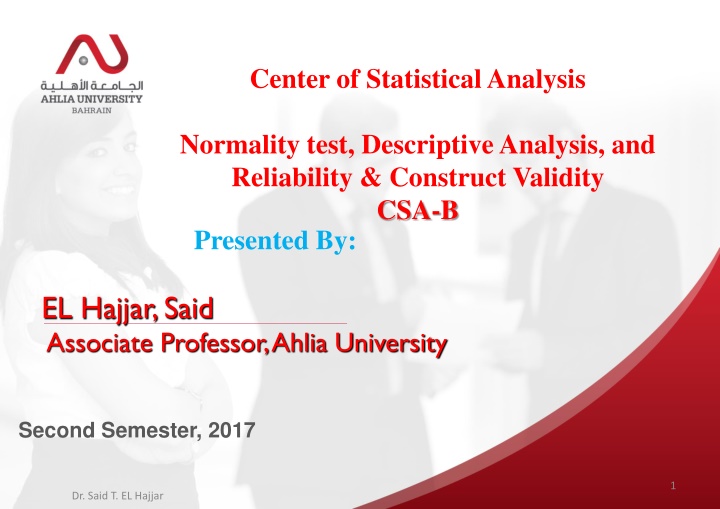
Center of Statistical Analysis Normality test, Descriptive Analysis, and Reliability & Construct Validity CSA-B Presented By: EL Hajjar, Said Associate Professor, Ahlia University Second Semester, 2017 1 Dr. Said T. EL Hajjar

Data Analysis Acceptable sample size for a given population size It is highly recommended to find the response rate before proceeding in any analysis. Response rate = ( number of received responses / total number of distributed questionnaire ) ; this sample response rate should be more than or equal to 30 % of parent data ( Sekaran, 2003). 2 1 ( ) z p p - Here are two methods to calculate the required sample size: 2 e = n 1- Calculation Method if population size is known 2 1 ( ) z p p + 1 2 e N N = Population size; e = acceptable margin of error for the mean to be estimated. 3% is a reasonable figure to be assumed as margin of error. (Krejcie and Morgan,1970) p = Percentage Value ( 0.5) Z = critical value (acceptable risk); Value of z is based on the risk that you choose ( ) ; it is determined through z-Table. Recommended values of are 5% or 1% risk . Dr. Said T. EL Hajjar 2

Data Analysis (Continued) Example Suppose that the number of distributed questionnaire is 400, and the number of received responses is 385. then: Response rate = ( number of received responses / total number of distributed questionnaire ) = 385 / 400 = 0. 9625, which is 96.25 % sample response rate 30% .Calculation Method Suppose N = 500, 95% confidence level(z= 1.96), and the margin of error is e = 0.03. ) 1 ( 2 = + N e 1 ( 5 . 0 ) 5 . 0 2 2 . 1 96 z p p 2 . 0 2 03 e = = 340 47 . 341 n ) 5 . 0 2 1 ( 2 ) . 1 + 96 1 ( 5 . 0 2 z p p 1 1 . 0 03 500 Dr. Said T. EL Hajjar 3

Data Analysis (Continued) Population Size Sample Size per Margin of Error 95% Confidence Level 3% 5% 10% 500 345 220 80 1,000 525 285 90 3,000 810 350 100 5,000 910 370 100 10,000 1,000 385 100 100,000+ 1,100 400 100 Dr. Said T. EL Hajjar 4

Data Analysis (Continued) Sample Size Table - The Research Advisors research-advisors.com/tools/SampleSize.htm Dr. Said T. EL Hajjar 5

Data Analysis 2) Acceptable sample size for an unknown population size n ( e ) 2 1 z p p = 2 Where the population is unknown, the sample size can be derived by computing the minimum sample size required for accuracy in estimating proportions by considering the standard normal deviation set at 95% confidence level ( z = 1.96), a sample proportion of 50% ( p = 0.5 ) a margin of error 5% ( e = 0.05). ( Mensah, 2014) Dr. Said T. EL Hajjar 6

Normality test Describe the balance of the distribution: Skewness and Kurtosis. - Skewness: Acceptable range for values is [-2, 2] - Kurtosis: Acceptable range for values is [-3, 3] Reference: (Hair et al., 2010). With small sample size, the impact of Skewness and Kurtosis might not make a significant difference in further analyses. Reference: (Tabachnick and Fidell, 2001). Dr. Said T. EL Hajjar 7

Normality test (case 1) (Continued) Data are normally Distributed Skewness Score [-2, 2 ] and Kurtosis Score [-3, 3 ] Dr. Said T. EL Hajjar 8

Normality test (case II ) (Continued) Data are approximately normally Distributed Although PP3 & SS3 Skewness Scores fell outside the range of [- 2, 2 ] and PP3 &TP2 Kurtosis Scores fell outside the range of [- 3, 3 ], there is no statistical reason to drop them. Due to the sample size, the impact of Skewness and Kurtosis might significant difference in further analyses (Tabachnick and Fidell, 2001). not make a Dr. Said T. EL Hajjar 9

Description of Data Frequency Table : Family Income in Dollars per year Frequency Percent Valid Percent Cumulative Percent Valid Less than 14 K 14K - 19,999 20K - 49,999 50K or more Total Missing System Total 2 1.6 1.6 1.6 8 52 62 124 4 128 6.3 40.6 48.4 96.9 3.1 100.0 6.5 41.9 50.0 100.0 8.1 50.0 100.0 10 Dr. Said T. EL Hajjar

Description of Data It analyzes the respondent s personal Information . Output (Age) Frequency: Count of interviews in survey. These counts are useful if you want to calculate different percentage categories. Percent: Percentages of all respondents, with those who did not answer or said they did not know included. Valid Percent: Percentages of all respondents who answered the question with an opinion on it. Respondents who did not answer or said they did not know are not included. Cumulative Percent :This adds up percentages from top to bottom as you go. It is just there to make the arithmetic easier. 11 Dr. Said T. EL Hajjar

Description of Data Frequency Table : Family Income in Dollars per year 124 out of the 128 parents have valid data. You can see the "valid percent" are slightly higher than the "percent" because the 4 missing cases have been removed from consideration. Note that sometimes you need to do some recalculating on your own. Here is an example from the Frequencies table above: "Eight percent of respondents reported their family income to be less than $19,999 per year." The 8% figure comes from adding the valid percent from two rows (1.6 for those less than 14K and 6.5 for those from 14 K to 19,999). In the final report, we recommend rounding percentages to the nearest whole number. We lose a little accuracy this way, but avoid frightening math-phobic people. So we would round 14.4 to 14 and 14.6 to 15. But which way would you round 14.5? Here is the rule of Thumb we follow: round .5 to the nearest even number. Therefore, 14.5 would round down to 14, but 15.5 would round up to 16, the nearest even number. In this way there is no systemic bias upward or downward. Frequency Percent Valid Percent Cumulative Percent Valid Less than 14 K 14K - 19,999 20K - 49,999 50K or more Total Missing System Total 2 1.6 1.6 1.6 8 52 62 124 4 128 6.3 40.6 48.4 96.9 3.1 100.0 6.5 41.9 50.0 100.0 8.1 50.0 100.0 12 Dr. Said T. EL Hajjar

Description of Data Age: Bar charts A bar graph (or bar chart) is perhaps common statistical display used by the media. A bar graph categorical data down by group, and represents these amounts by using bars of different lengths. It uses either the individuals in each group (also called the frequency) or the percentage in each group (called the relative frequency). the most data breaks number of 13 Dr. Said T. EL Hajjar

Description of Data This particular bar graph shows how much money is spent on transportation for people in different household-income groups. It appears that as household income increases, the total expenditures on transportation also increase. This makes sense, because the more money people have, the more they have available to spend. But would the bar graph change if you looked at transportation expenditures not in terms of total dollar amounts, but as the percentage of household income? The households in the first group make less than $5,000 a year and have to spend $2,500 of it on transportation. (Note: The label reads 2.5, but because the units are in thousands of dollars, the 2.5 translates into $2,500.) 14 Dr. Said T. EL Hajjar

Description of Data This $2,500 represents 50% of the annual income of those who make $5,000 per year; the percentage of the total income is even higher for those who make less than $5,000 per year. The households earning $30,000 $40,000 per year pay $6,000 per year on transportation, which is between 15% and 20% of their household income. So, although the people making more money spend transportation, they don t spend more as a percentage of their Depending on how expenditures, the bar graph can tell two somewhat different stories. more dollars on total you income. look at 15 Dr. Said T. EL Hajjar

Description of Data Another point to check out is the groupings on the graph. The categories for household income as shown aren t equivalent. For example, each of the first four bars represents household incomes in intervals of $5,000, but the next three groups increase by $10,000 each, and the last group contains every household making more than $50,000 per year. Bar graphs using different-sized intervals to represent numerical values (as indicated in the image) make true comparisons between groups more difficult. (However, the government probably has its reasons for reporting the numbers this way; for example, this may be the way income is broken down for tax-related purposes.) 16 Dr. Said T. EL Hajjar

Description of Data One last thing: Notice that the numerical groupings in the image overlap on the boundaries. For example, $30,000 appears in both the 5th and 6th bars of the graph. So, if you have a household income of $30,000, which bar do you fall into? This kind of overlap appears quite frequently in graphs, but you need to know how the borderline values are being treated. For example, the rule may be Any data lying exactly on a boundary value automatically goes into the bar to its immediate right. (Looking at the image, that puts a household with a $30,000 income into the 6th bar rather than the 5th.) 17 Dr. Said T. EL Hajjar

Measuring Data Central tendency refers to the idea that there is one number that best summarizes the entire set of measurements, a number that is in some way "central" to the set. The mode is the measurement that has the greatest frequency, the one you found the most of. Although it isn't used that much, it is useful when differences are rare or when the differences are non numerical. The prototypical example of something is usually the mode. The mode for our example is 4. It is the grade with the most people (4). 18 Dr. Said T. EL Hajjar

Measuring Data The median is the number at which half your measurements are more than that number and half are less than that number. The median is actually a better measure of centrality than the mean if your data are not normally distributed. The median for our example is 3.00. Half the people scored lower, and half higher (and one exactly). The mean is just the average. This is the most used measure of central tendency, because of its mathematical qualities. It works best if the data is normally distributed. One interesting thing about the mean is that it represents the expected value if the distribution of measurements were random! The mean for our example is 3.03. 19 Dr. Said T. EL Hajjar

Measuring Data Standard Deviation Standard deviation can be difficult to interpret as a single number on its own. Basically, a small standard deviation means that the values in a statistical data set are close to the mean of the data set, on average, and a large standard deviation means that the values in the data set are farther away from the mean, on average. The standard deviation measures how concentrated the data are around the mean; the more concentrated, the smaller the standard deviation. A small standard deviation can be a goal in certain situations where the results are restricted, for example, in product manufacturing and quality control. A particular type of car part that has to be 2 centimeters in diameter to fit properly had better not have a very big standard deviation during the manufacturing process. A big standard deviation in this case would mean that lots of parts end up in the trash because they don t fit right; either that or the cars will have problems down the road 20 Dr. Said T. EL Hajjar

Measuring Data Standard Deviation But in situations where you just observe and record data, a large standard deviation isn t necessarily a bad thing; it just reflects a large amount of variation in the group that is being studied. For example, if you look at salaries for everyone in a certain company, including everyone from the student intern to the CEO, the standard deviation may be very large. On the other hand, if you narrow the group down by looking only at the student interns, the standard deviation is smaller, because the individuals within this group have salaries that are less variable. The second data set isn t better, it s just less variable. 21 Dr. Said T. EL Hajjar

Standard Deviations Same mean, but different standard deviations: Data A Mean = 15.5 s = 3.338 11 12 13 14 15 16 17 18 19 20 21 Data B Mean = 15.5 s = .9258 11 12 13 14 15 16 17 18 19 20 21 Data C Mean = 15.5 s = 4.57 11 12 13 14 15 16 17 18 19 20 21 Dr Saeed Hajjar Chap 3-22

Measuring Data (Continued) Descriptive statistics - Shows the perceptions of respondents to variables. As shown, Respondents revealed that SS is the first important factor that may lead to influence the dependent variable (TP)( mean = 3.1314, Std. Deviation = 1.01511).The least important factor is PP( mean = 3.1257, Std. Deviation = 1.03706). Among the variables, the most important effective factor in the model is TP (Mean=3.3714, Std. Deviation =1.26132). Dr. Said T. EL Hajjar 23

Activity 1: Reliability & Construct Validity We need to study the reliability and validity of the constructs and items in this model. Note that here we use 10 -30% of the collected dataset. 24 Dr. Said T. EL Hajjar

Activity 1 (Case I ) Assume the following outputs: There is statistical reason to drop out the items PP3 and PP5 25 Dr. Said T. EL Hajjar

Activity 1 (Case II ) Assume the following outputs: There is no statistical reason to drop out the items PP3 and PP5 26 Dr. Said T. EL Hajjar

Activity 1 (Case III ) Assume the following outputs: There is no statistical reason to drop out the items PP3 and PP5 27 Dr. Said T. EL Hajjar

End THANK YOU 28 Dr. Said T. EL Hajjar