Analysis of Variance (ANOVA)
ANOVA, or Analysis of Variance, is a statistical method used to compare means of multiple groups based on a categorical variable. It helps evaluate hypotheses regarding group means, with one-way and two-way ANOVA being common variations. The process involves calculating between-groups (SSB) and within-groups (SSW) variations to explain the total variation in the data. The F-statistic is used to test for differences in means, following the null hypothesis that all group means are equal. The F-distribution plays a key role in hypothesis testing for ANOVA, with parameters df1 and df2 representing degrees of freedom. Explore ANOVA further through practical examples and applications.

Download Presentation

Please find below an Image/Link to download the presentation.
The content on the website is provided AS IS for your information and personal use only. It may not be sold, licensed, or shared on other websites without obtaining consent from the author.If you encounter any issues during the download, it is possible that the publisher has removed the file from their server.
You are allowed to download the files provided on this website for personal or commercial use, subject to the condition that they are used lawfully. All files are the property of their respective owners.
The content on the website is provided AS IS for your information and personal use only. It may not be sold, licensed, or shared on other websites without obtaining consent from the author.
E N D
Presentation Transcript
Statistical Data Analysis Prof. Dr. Nizamettin AYDIN naydin@yildiz.edu.tr http://www3.yildiz.edu.tr/~naydin 1
Analysis of Variance (ANOVA) 2
ANOVA The process of evaluating hypotheses regarding the group means of multiple populations is called the Analysis of Variance (ANOVA). ANOVA models generalize the t-test and are used to compare the means of multiple groups identified by a categorical variable with more than two possible categories. Since we are only considering one factor only, this method is specifically called one- way ANOVA. An ANOVA with two factors is called a two-way ANOVA. In general, the between-groups variation is denoted as SSBand calculated by ? ??(?? ?)2 ???= ?=1 where k is the number of groups 3
ANOVA The within-groups variation is denoted as SSWand calculated by ? ?? (??? ??)2 ???= ?=1 ?=1 We measure the total variation in Y by ? ?? (??? ?)2 ?? = ?=1 ?=1 The total variation SS is equal to the sum of the between-groups variation SSBand the within-groups variation SSW, SS = SSB+SSW. The total variation can be attributed partly to the variation within groups and partly to the variation between groups. SSBis interpreted as the part of total variation SS that is associated with (and can be explained by) the factor variable X (e.g., syndrome type). In contrast, SSWis regarded as the unexplained part of total variation and is regarded as random. 4
ANOVA Let us denote the overall population mean of Y as and group- specific population means as 1, . . . , 4. Then we can express the null hypothesis of no difference in means between the groups as H0 : 1= 2= 3= 4= The alternative hypothesis HAis that at least one of the group means iis different from the mean . The test statistic for examining the null hypothesis is called F- statistic (more specifically, ANOVA F -statistic) and is defined as ? =???/(? 1) ???/(? ?) where n is the total sample size, and k is the number of groups. The numerator is called the mean square for groups, and the denominator is called the mean square error (MSE). 5
ANOVA For the one-way ANOVA, the F-statistic has F(df1= k 1, df2= n k) distribution under the null hypothesis (i.e., assuming that the null hypothesis is true). The F-distribution, which is a continuous probability distribution, is very important for hypothesis testing. It is specified by two parameters, df1and df2, and is denoted as F(df1, df2). We refer to df1and df2as the numerator degrees of freedom and denominator degrees of freedom, respectively. Both parameters must be positive. 6
ANOVA The following figure shows the pdf of F-distribution for different values of df1and df2. 7
Example As an example, we analyze the Cushings data set, which is available from the MASS package. Cushing s syndrome is a hormone disorder associated with high level of cortisol secreted by the adrenal gland. The Type variable in the data set shows the underlying type of syndrome, which can be one of four categories: adenoma (a), bilateral hyperplasia (b), carcinoma (c), unknown (u). 8
Example Objective is to find whether the four groups are different with respect to urinary excretion rate of Tetrahydrocortisone. We denote by Y the urinary excretion rate of Tetrahydrocortisone and by X the Type variable, where X = 1 for Type = a, X = 2 for Type = b, X = 3 for Type = c, and X = 4 for Type = u. Then, our objective could be defined as investigating whether the mean of the response variable Y differs for different values (levels) of the factor X. 9
Example Denote the individual observations as yij: the urinary excretion rate of Tetrahydrocortisone of the jth individual in group i. Total number of observations is n = 27, The number of observations in each group is n1= 6, n2= 10, n3= 5, and n4= 6. The overall (for all groups) observed sample mean for the response variable is ? = 10.46. We also find the group specific means, by clicking (in R-Commander) Statistics Summaries Numerical summaries ?1= 3.0, ?2= 8.2, ?3= 19.7, and ?4= 14.0. The degrees of freedom parameters are df1= 4 1= 3 and df2= 27 4 = 23. 10
Example SSB= 893.5 and SSW= 2123.6. The observed value of F-statistic is f = 3.2 given under the column labeled F value. The resulting p-value is then 0.04. Therefore, we can reject H0at 0.05 significance level (but not at 0.01) and conclude that the differences among group means for urinary excretion rate of Tetrahydrocortisone are statistically significant (at 0.05 level). 11
Example For plotting the F(3, 23) distribution using R-Commander, click Distribution Continuous distributions F distribution Plot F distribution. Set the Numerator degrees of freedom to 3 and the Denominator degrees of freedom to 23. The density plot of F(3, 23)-distribution. This is the distribution of F-statistic for the Cushings data assuming that the null hypothesis is true. The observed value of the test statistic is = 3.2, and the corresponding p-value is shown as the shaded area above 3.2 f 12