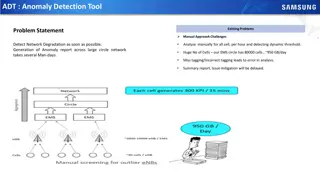
Anomaly Detection: Understanding Outliers in Data Mining
Anomaly detection is crucial for identifying outliers in datasets, such as credit card fraud or ozone depletion in historical data. This process involves finding data points that deviate significantly from the norm, posing challenges like unsupervised validation and the imbalance between normal and abnormal observations.

Download Presentation

Please find below an Image/Link to download the presentation.
The content on the website is provided AS IS for your information and personal use only. It may not be sold, licensed, or shared on other websites without obtaining consent from the author.If you encounter any issues during the download, it is possible that the publisher has removed the file from their server.
You are allowed to download the files provided on this website for personal or commercial use, subject to the condition that they are used lawfully. All files are the property of their respective owners.
The content on the website is provided AS IS for your information and personal use only. It may not be sold, licensed, or shared on other websites without obtaining consent from the author.
E N D
Presentation Transcript
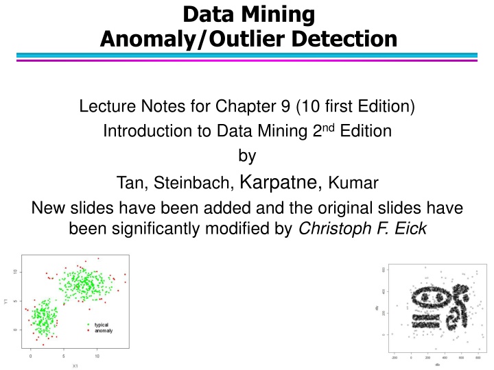
Data Mining Anomaly/Outlier Detection Lecture Notes for Chapter 9 (10 first Edition) Introduction to Data Mining 2nd Edition by Tan, Steinbach, Karpatne, Kumar New slides have been added and the original slides have been significantly modified by Christoph F. Eick
Lecture Organization 0. Anomaly/Outlier Detection 1. Graphic-based Approaches 2. Model-based Statistical Approaches 3. One-Class SVM Approach 4. Distance-Based Approaches http://tse1.mm.bing.net/th?id=OIP.M475b8b96cd2de276a042f9c263e3ddfbH0w=163h=109c=7rs=1qlt=90pid=3.1rm=2 Anomaly Detection Coverage in COSC 4355 Please note, 7/8 of an iceberg are under water! 4/12/2018 Eick, Tan,Steinbach,Kapatne, Kumar COSC 4335: Data Mining
0. Anomaly/Outlier Detection What are anomalies/outliers? The set of data points that are considerably different than the remainder of the data Variants of Anomaly/Outlier Detection Problems Given a database D, find all the data points x D with anomaly scores greater than some threshold t Given a database D, find all the data points x D having the top-n largest anomaly scores f(x) Given a database D, containing mostly normal (but unlabeled) data points, and a test point x, compute the anomaly score of x with respect to D Applications: Credit card fraud detection, telecommunication fraud detection, network intrusion detection, fault detection, data cleaning, sensor fusion, 4/12/2018 Eick, Tan,Steinbach,Kapatne, Kumar COSC 4335: Data Mining
Importance of Anomaly Detection Ozone Depletion History In 1985 three researchers (Farman, Gardinar and Shanklin) were puzzled by data gathered by the British Antarctic Survey showing that ozone levels for Antarctica had dropped 10% below normal levels Why did the Nimbus 7 satellite, which had instruments aboard for recording ozone levels, not record similarly low ozone concentrations? The ozone concentrations recorded by the satellite were so low they were being treated as outliers by a computer program and discarded! Sources: http://exploringdata.cqu.edu.au/ozone.html http://www.epa.gov/ozone/science/hole/size.html 4/12/2018 Eick, Tan,Steinbach,Kapatne, Kumar COSC 4335: Data Mining
Anomaly Detection Challenges How many outliers are there in the data? Method is unsupervised Validation can be quite challenging (just like for clustering) Finding needle in a haystack Working assumption: There are considerably more normal observations than abnormal observations (outliers/anomalies) in the data 4/12/2018 Eick, Tan,Steinbach,Kapatne, Kumar COSC 4335: Data Mining
Anomaly Detection Schemes General Steps Build a profile of the normal behavior Profile can be patterns or summary statistics for the overall population Use the normal profile to detect anomalies Anomalies are observations whose characteristics differ significantly from the normal profile Types of anomaly detection schemes 1. Graphical 2. Model-based, relying on parametric models 3. One-Class SVM Approach 4. Distance-based 4/12/2018 Eick, Tan,Steinbach,Kapatne, Kumar COSC 4335: Data Mining
1. Graphical Approaches Idea: user identifies outliers by visual inspection Scatter plot (2-D), Spin plot (3-D) Limitations Time consuming Subjective 4/12/2018 Eick, Tan,Steinbach,Kapatne, Kumar COSC 4335: Data Mining
Convex Hull Method Extreme points are assumed to be outliers Use convex hull method to detect extreme values http://cgm.cs.mcgill.ca/~godfried/teaching/project s97/belair/alpha.html 4/12/2018 Eick, Tan,Steinbach,Kapatne, Kumar COSC 4335: Data Mining
Box-Plot Approach for Outlier Detection outlier 1.5*IQR IQR Mixture of a graphical and a statistical approach Observations that are more than IQR (e.g. =1.5) above or below the inter-quantile range are outliers. Decent approach for 1D/single attribute outlier detection! Sad news: Cannot be used for multi-variate data! 4/12/2018 Eick, Tan,Steinbach,Kapatne, Kumar COSC 4335: Data Mining
Outlier Detection Example1 4/12/2018 Eick, Tan,Steinbach,Kapatne, Kumar COSC 4335: Data Mining
Outlier Detection Example2 4/12/2018 Eick, Tan,Steinbach,Kapatne, Kumar COSC 4335: Data Mining
Anomaly/Outlier Detection (Second Introduction) What are anomalies/outliers? The set of data points that are considerably different than the remainder of the data Natural implication is that anomalies are relatively rare One in a thousand occurs often if you have lots of data Context is important, e.g., freezing temps in July Can be important or a nuisance 10 foot tall 2 year old Unusually high blood pressure 4/12/2018 Eick, Tan,Steinbach,Kapatne, Kumar COSC 4335: Data Mining
Causes of Anomalies Data from different classes Measuring the weights of oranges, but a few grapefruit are mixed in Natural variation Unusually tall people Data errors 200 pound 2 year old 4/12/2018 Eick, Tan,Steinbach,Kapatne, Kumar COSC 4335: Data Mining
Object vs. Attribute Anomalies Many anomalies are defined in terms of a single attribute Height Shape Color Object anomalies are harder to identify as objects are usually described by multiple attributes Can be hard to find an anomaly using all attributes Noisy or irrelevant attributes Object is only anomalous with respect to some attributes However, an object may not be anomalous in any one attribute 4/12/2018 Eick, Tan,Steinbach,Kapatne, Kumar COSC 4335: Data Mining
General Issues: Anomaly Scoring Many anomaly detection techniques provide only a binary categorization An object is an anomaly or it isn t This is especially true of classification-based approaches Other approaches assign a score to all points This score measures the degree to which an object is an anomaly This allows objects to be ranked In general, this is the preferable approach However, in the end, you often need a binary decision Should this credit card transaction be flagged? Still useful to have a score How many anomalies are there? 4/12/2018 Eick, Tan,Steinbach,Kapatne, Kumar COSC 4335: Data Mining
Model-Based Anomaly Detection Build a model for the data and see Unsupervised Anomalies are those points that don t fit well Anomalies are those points that distort the model Examples: Statistical distribution Clusters Regression Geometric Graph Supervised Anomalies are regarded as a rare class Need to have training data 4/12/2018 Eick, Tan,Steinbach,Kapatne, Kumar COSC 4335: Data Mining
Additional Anomaly Detection Techniques Proximity-based Anomalies are points far away from other points Can detect this graphically in some cases Density-based Low density points are outliers Pattern matching Create profiles or templates of atypical but important events or objects Algorithms to detect these patterns are usually simple and efficient 4/12/2018 Eick, Tan,Steinbach,Kapatne, Kumar COSC 4335: Data Mining
2. Model-based Statistical Approaches Fit a parametric model M to the data, capturing the distribution of the data (e.g., normal distribution) Apply a statistical test that depends on Data distribution Parameter of distribution (e.g., mean, variance) Number of expected outliers (confidence limit) Alternatively, rank points by their likelihood with respect to M Data Density Function 4/12/2018 Eick, Tan,Steinbach,Kapatne, Kumar COSC 4335: Data Mining
Normal Distributions One-dimensional Gaussian 8 7 0.1 6 0.09 5 0.08 4 Two-dimensional Gaussian 0.07 3 0.06 2 0.05 1 y 0.04 0 0.03 -1 0.02 -2 -3 0.01 -4 probability density -5 -4 -3 -2 -1 0 1 2 3 4 5 x 19 4/12/2018 Eick, Tan,Steinbach,Kapatne, Kumar COSC 4335: Data Mining
Skipped in 2018 Grubbs Test Detect outliers in univariate data Assume data comes from normal distribution Detects one outlier at a time, remove the outlier, and repeat H0: There is no outlier in data HA: There is at least one outlier Grubbs test statistic: G max X X = s Reject H0 if: 2 t ) 1 N ( N G ( / + , 2 ) N N t 2 2 N ( / , 2 ) N N 4/12/2018 Eick, Tan,Steinbach,Kapatne, Kumar COSC 4335: Data Mining
Assigment4-like Dataset 4/12/2018 Eick, Tan,Steinbach,Kapatne, Kumar COSC 4335: Data Mining
Density Plot for Assigment4-like Dataset Remark: Using a model-based approach points on the same density contour line should have the same likelihood to be outliers with respect to the underlying statistical model M. 4/12/2018 Eick, Tan,Steinbach,Kapatne, Kumar COSC 4335: Data Mining
Another Better Density Contour Plot 4/12/2018 Eick, Tan,Steinbach,Kapatne, Kumar COSC 4335: Data Mining
Statistical Approaches for Assignment4 1. Fit a model M to the dataset D; e.g. A Bivariate Gaussian Model A Bivariate Gaussian Mixture Model by running the EM clustering algorithm; see: https://brilliant.org/wiki/gaussian-mixture-model/ 2. Plug each point p into the density function dM of model M and compute dM(p) or preferably log(dM(p)), called the log likelihood of p, and add this value as in a new column ols ( outlier score ) to D obtaining D the smaller this value is the more likely p is an outlier with respect M. 3. Sort D in ascending order the first record is the record with the smallest value for log(dM(p)) 4. Perform the remaining tasks using D GMM-Model 4/12/2018 Eick, Tan,Steinbach,Kapatne, Kumar COSC 4335: Data Mining
General Idea EM Algorithm EM Algorithm Gaussian Mixture Models: http://research.stowers.org/mcm/efg/R/Statistics/MixturesOfDistributions/index.htm http://pypr.sourceforge.net/mog.html http://scikit-learn.org/stable/modules/mixture.html http://cs229.stanford.edu/notes/cs229-notes8.pdf Works like K-means 25 4/12/2018 Eick, Tan,Steinbach,Kapatne, Kumar COSC 4335: Data Mining
Parameter of K-Means/GMM Models K-means models are characterized by k centroids EM/Gaussian Mixture Models are characterized by k Gaussian with each Gaussian characterized by: Weight of the particular Gaussian Mean value Covariance Matrix EM-style algorithms: E-Step: Assign objects to clusters (deterministic in the case of K-means; probabilistic in the case of EM) M-Step: updates the model parameters (e.g. centroids in the case of K-means; the mixture parameter in the case of EM) Repeat sequences of E-M steps until there is some convergence Start with an initial assignment of objects to clusters 4/12/2018 Eick, Tan,Steinbach,Kapatne, Kumar COSC 4335: Data Mining
Likelihood-Based Removal Approach skip Assume the data set D contains samples from a mixture of two probability distributions: M (majority distribution) A (anomalous distribution) General Approach: Initially, assume all the data points belong to M Let Lt(D) be the log likelihood of D at time t For each point xt that belongs to M explore the affect of moving it to A Let Lt+1 (D) be the new log likelihood after removing xt Compute the difference, = Lt+1(D) Lt (D) If > c (some threshold), then xt is declared as an anomaly and moved permanently from M to A 4/12/2018 Eick, Tan,Steinbach,Kapatne, Kumar COSC 4335: Data Mining
Limitations of Statistical Approaches Most of the statistical tests are for a single attributes In many cases, data distribution/model may not be known For high dimensional data, it may be difficult to estimate the true density function. However, mixtures of Gaussians and conjunction with EM have been successfully used in practice for some outlier detection tasks that involve multi-variate data. As alternative to parametric density estimation, non-parametric density-based approaches, such as kernel density estimation have shown some promise; see: https://en.wikipedia.org/wiki/Kernel_density_estimation (maybe to be discussed in the next lecture!). However, these approaches just provide you with estimated densities but not with a true density function density function; therefore, they are not truly model based, but rather just density-based approaches. 4/12/2018 Eick, Tan,Steinbach,Kapatne, Kumar COSC 4335: Data Mining
Density-based: LOF approach For each point, compute the density of its local neighborhood; e.g. use DBSCAN s approach In anomaly detection, the local outlier factor (LOF) is an algorithm proposed by Markus M. Breunig, Hans-Peter Kriegel, Raymond T. Ng and J rg Sander in 2000 for finding anomalous data points by measuring the local deviation of a given data point with respect to its neighbours.[1] Outliers are points with largest LOF value (measured as point- density/neighbor densities) In the NN approach, p2 is not considered as outlier, while LOF approach find both p1 and p2 as outliers; moreover, some/all points in cluster C1 might be considered as outliers! p2 p1 4/12/2018 Eick, Tan,Steinbach,Kapatne, Kumar COSC 4335: Data Mining
Relative Density Outlier Scores 6.85 6 C 5 4 1.40 D 3 1.33 2 A 1 Outlier Score 30 4/12/2018 Eick, Tan,Steinbach,Kapatne, Kumar COSC 4335: Data Mining
Strengths/Weaknesses of Density-Based Approaches Simple Expensive O(n2) Sensitive to parameters Density becomes less meaningful in high- dimensional space 4/12/2018 Eick, Tan,Steinbach,Kapatne, Kumar COSC 4335: Data Mining
3. One-Class SVM Approach for Outlier Detection Consider a sphere with center a and radius R Minimize R and the error resulting from points outside the sphere their error is their distance to the sphere. Lowercase greek xiletter, pronounced ksi C + 2 t min R t subject to + 2 t t t x , 0 a R error More information: http://rvlasveld.github.io/blog/2013/07/12/introduction-to-one-class-support-vector-machines/ 4/12/2018 Eick, Tan,Steinbach,Kapatne, Kumar COSC 4335: Data Mining
One Class SVM with Kernel Functions Again kernel functions/mapping to a higher dimensional space can be employed in which case the class boundary shapes change as depicted. 4/12/2018 Eick, Tan,Steinbach,Kapatne, Kumar COSC 4335: Data Mining
4. Distance-based Approaches Data is represented as a vector of features Three major approaches 1. K-Nearest-neighbor based 2. Density-based approaches, relying on non- parametric density estimation techniques 3. Clustering based 4/12/2018 Eick, Tan,Steinbach,Kapatne, Kumar COSC 4335: Data Mining
Nearest-Neighbor Based Approach Approach: Compute the distance between every pair of data points There are various ways to define outliers: Data points for which there are fewer than p neighboring points within a distance r The top n data points whose distance to the kth nearest neighbor is greatest The top n data points whose average distance to the k nearest neighbors is greatest 4/12/2018 Eick, Tan,Steinbach,Kapatne, Kumar COSC 4335: Data Mining
One Nearest Neighbor - One Outlier D 2 1.8 1.6 1.4 1.2 1 0.8 0.6 0.4 4/12/2018 Eick, Tan,Steinbach,Kapatne, Kumar COSC 4335: Data Mining
One Nearest Neighbor - Two Outliers 0.55 D 0.5 0.45 0.4 0.35 0.3 0.25 0.2 0.15 0.1 0.05 4/12/2018 Eick, Tan,Steinbach,Kapatne, Kumar COSC 4335: Data Mining
Five Nearest Neighbors - Small Cluster 2 D 1.8 1.6 1.4 1.2 1 0.8 0.6 0.4 4/12/2018 Eick, Tan,Steinbach,Kapatne, Kumar COSC 4335: Data Mining
Five Nearest Neighbors - Differing Density D 1.8 1.6 1.4 1.2 1 0.8 0.6 0.4 0.2 4/12/2018 Eick, Tan,Steinbach,Kapatne, Kumar COSC 4335: Data Mining
4. Clustering-Based Approaches Clustering-based Outlier: An object is a cluster-based outlier if it does not strongly belong to any cluster For prototype-based clusters, an object is an outlier if it is not close enough to a cluster center For density-based clusters, an object is an outlier if its density is too low For graph-based clusters, an object is an outlier if it is not well connected Other issues include the impact of outliers on the clusters and the number of clusters 4/12/2018 Eick, Tan,Steinbach,Kapatne, Kumar COSC 4335: Data Mining
Clustering-Based Basic Idea: Run a clustering algorithm, objects that do not rely belong to any cluster are considered to be outliers! Problem what parameters should I choose for the algorithm; e.g. we could just run DBSCAN and report the outliers! Rule of Thumb: Less than x% of the data should be outliers (with x typically chosen between 0.1 and 10); x might be determined with other methods; e.g. statistical tests. Needs Tweaking for Assignment4 as this approach does not produce a number! 4/12/2018 Eick, Tan,Steinbach,Kapatne, Kumar COSC 4335: Data Mining
Distance of Points from Closest Centroids 4.5 4.6 4 C 3.5 3 2.5 D 0.17 2 1.5 1.2 1 A 0.5 Outlier Score 4/12/2018 Eick, Tan,Steinbach,Kapatne, Kumar COSC 4335: Data Mining
Assigment4-like Dataset 4/12/2018 Eick, Tan,Steinbach,Kapatne, Kumar COSC 4335: Data Mining
R-Code Used to Create the Complex9_gn16 Displays #Code for Scatter Plots setwd("C:/Users/8yetula8\\Desktop") a<-read.csv("complex9_gn16.txt") d<-data.frame(x=a[,1],y=a[,2],class=factor(a[,3])) plot(d$x,d$y) require("lattice") require("ggplot2") xyplot(y ~ x | class, d, groups=d$class, pch=20) ggplot(d, aes(x=x, y=y, colour=class))+ geom_point() ggplot(d, aes(x = x, y = y)) + geom_point() + facet_grid(~class) ggplot (d, aes (x = x, y = y, colour = class)) + stat_density2d () p <- ggplot(d, aes(x = x,y = y)) p+geom_point()+geom_density2d() #another approach; seems to get more meaningful contours require("MASS") require("KernSmooth") y <- cbind(d$x, d$y) #this apporach uses kernel density estimation; est <- bkde2D(y, bandwidth=c(20, 18)) contour(est$x1, est$x2, est$fhat) persp(est$fhat) 4/12/2018 Eick, Tan,Steinbach,Kapatne, Kumar COSC 4335: Data Mining
Brainstorming for Assignment4 Approaches Potential Approaches: Density-based: OLS value is the density of that point; dataset is inversely sorted by the OLS value. How do I measure the density? Wrap a radius r around the point p and count the number of points Use non-parametric kernel density estimation techniques Distance-based: Compute the k-nearest neighbor distance for each point; possibly make it more sophisticated; might refine this approach by using multiple k-nearest neighbor distances. Clustering-based; e.g. use DBSCAN clusters; ols-score is the distance of a point to a point of the nearest cluster; for points inside a cluster it is (the inverse distance to the cluster center); use K-means and use each points distance to its clusters centroid as the OLS score One Class SVM (not so clear; how do I get an OLS scores) Model-based; however, using single Gaussian will not work well for our dataset Mixture of Gaussians are promising, but not easy to use 4/12/2018 Eick, Tan,Steinbach,Kapatne, Kumar COSC 4335: Data Mining
Another Better Density Contour Plot 4/12/2018 Eick, Tan,Steinbach,Kapatne, Kumar COSC 4335: Data Mining


")