Applications of Time-Frequency Analysis for Filter Design

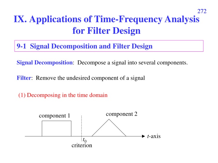
272 IX. Applications of Time-Frequency Analysis for Filter Design 9-1 Signal Decomposition and Filter Design Signal Decomposition: Decompose a signal into several components. Filter: Remove the undesired component of a signal (1) Decomposing in the time domain component 2 component 1 t-axis t0 criterion

273 (2) Decomposing in the frequency domain ( ) sin(4 x t t = ) cos(10 + ) t -5 -2 2 5 f-axis Sometimes, signal and noise are separable in the time domain (1) without any transform Sometimes, signal and noise are separable in the frequency domain (2) using the FT (conventional filter) = ( ) ( ( )) ( ) i x t IFT FT x t H f o If signal and noise are not separable in both the time and the frequency domains (3) Using the fractional Fourier transform and time-frequency analysis

274 criterion in the time domain cutoff line perpendicular to t-axis f-axis cutoff line = t0 t-axis t-axis t0 criterion in the frequency domain cutoff line perpendicular to f-axis f-axis cutoff line f0 f-axis= f0 t-axis

x(t) = triangular signal + chirp noise 0.3exp[j 0.5(t 4.4)2] 275 signal + noise FT 1 1 0.5 0.5 0 0 -0.5 -0.5 -10 -5 0 5 10 -10 -5 0 5 10 reconstructed signal 3 FRFT 1 = -arccot(1/2 ) 2 0.5 1 0 0 -0.5 -10 -5 0 5 10 -10 -5 0 5 10

x(t) = triangular signal + chirp noise 0.3exp[j 0.5(t 4.4)2] 276 2 1.5 1 0.5 f-axis 0 -0.5 -1 -1.5 -2 -8 -6 -4 -2 0 2 4 6 t-axis 8

277 Decomposing in the time-frequency distribution If x(t) = 0 for t < T1and t > T2 ( ) , 0 x W t f = for t < T1and t > T2(cutoff lines perpendicular to t-axis) If X( f ) = FT[x(t)] = 0 for f < F1and f > F2 for f < F1and f > F2(cutoff lines parallel to t-axis) What are the cutoff lines with other directions? ( ) W t f = , 0 x with the aid of the FRFT, the LCT, or the Fresnel transform

278 Filter designed by the fractional Fourier transform ( ) ( ) o F F i x t O O x t ( ) = = H u ( ) ( ( )) ( ) i x t IFT FT x t H f o O means the fractional Fourier transform: F ( ) x t dt e e e 2 csc cot ( ) u 2 j j t t 2 u = cot j ( ) x t 1 cot O j F f-axis Signal noise noise noise Signal Signal FRFT FRFT t-axis cutoff line cutoff line

279 ( ) ( ) ( ) = x t O O x t H u o F F i 1 0 u u u u ( ) ( ) ( ) = + H u S u u If 0 = H u 0 0 1 0 u u u u ( ) ( ) ( ) 0 = = H u S u u H u If 0 0 S(u): Step function 0 (1) cutoff line f-axis (2) u0 cutoff line ( )

280 Effect of the filter designed by the fractional Fourier transform (FRFT): Placing a cutoff line in the direction of ( sin , cos ) = 0 = 0.15 = 0.35 = 0.5 (time domain) (FT)

281 f-axis (0, f1) desired part cutoff line . undesired part (-t0, 0) . t-axis (t1, 0) undesired part cutoff line (0, -f0) = ? u0= ?

282 The Fourier transform is suitable to filter out the noise that is a combination of sinusoid functions exp(jn1t). The fractional Fourier transform (FRFT) is suitable to filter out the noise that is a combination of higher order exponential functions exp[j(nk tk+ nk-1 tk-1+ nk-2 tk-2+ . + n2 t2+ n1 t)] For example: chirp function exp(jn2 t2) With the FRFT, many noises that cannot be removed by the FT will be filtered out successfully.

283 Example (I) 4 4 10 real part imaginary part 5 2 2 0 0 0 -5 -2 -2 -10 -10 0 10 -10 0 10 -10 0 10 t axis (a) Signal s(t) (b) f(t) = s(t) + noise (c) WDF of s(t) ( ) s t ( ) = 2 2cos 5 exp( /10) t t 2 2 2 + = + + 0.23 0.3 8.5 0.46 9.6 j t j t j t j t j t ( ) 0.5 0.5 0.5 n t e e e

284 10 10 10 5 5 5 0 0 0 -5 -5 -5 -10 -10 -10 -10 (d) WDF of f(t) (e) GT of s(t) (f) GT of f(t) 0 10 -10 0 10 -10 0 10 GT: Gabor transform, WDF: Wigner distribution function horizontal: t-axis, vertical: -axis

285 GWT: Gabor-Wigner transform 10 10 10 5 5 5 L3 0 0 0 L1 L2 -5 -5 -5 -10 -10 -10 -10 0 10 L4 -10 (g) GWT of f(t) (h) Cutoff lines on GT 0 10 -10 (i) Cutoff lines on GWT 0 10 FrFT order

286 10 10 10 5 5 5 0 0 0 -5 -5 -5 -10 -10 -10 L1 L2 -10 (j) performing the FRFT 0 10 -10 0 10 -10 (e) Cutoff lines corresponding to the high pass filter (k) High pass filter (l) GWT after filter 0 10 (d) GWT of (a) (f) GWT of (c) (performing the FRFT) and calculate the GWT 2 2 1 1 0 0 mean square error (MSE) = 0.1128% -1 -1 -2 -2 -10 0 10 -10 0 10 (h) Recovered signal (real part) and the origianl signal (g) Recovered signal (m) recovered signal (n) recovered signal (green) and the original signal (blue)

287 Example (II) 3 7 . 0 exp( . 0 j 032 4 . 3 j ) t t Signal + 10 3 2 5 2 1 0 1 -5 0 0 -10 -1 -10 (a) Input signal (b) Signal + noise (c) WDF of (b) 0 10 -10 0 10 -10 0 10 10 10 2 MSE = 0.3013% 5 5 0 0 1 -5 -5 0 -10 -10 -10 (d) Gabor transform of (b) (e) GWT of (b) (f) Recovered signal 0 10 -10 0 10 -10 0 10

288 [Important Theory]: Using the FT can only filter the noises that do not overlap with the signals in the frequency domain (1-D) In contrast, using the FRFT can filter the noises that do not overlap with the signals on the time-frequency plane (2-D)

289 [ ] Q1: time-frequency distribution filter signal decomposition Q2: Cutoff lines

290 [Ref] Z. Zalevsky and D. Mendlovic, Fractional Wiener filter, Appl. Opt., vol. 35, no. 20, pp. 3930-3936, July 1996. [Ref] M. A. Kutay, H. M. Ozaktas, O. Arikan, and L. Onural, Optimal filter in fractional Fourier domains, IEEE Trans. Signal Processing, vol. 45, no. 5, pp. 1129-1143, May 1997. [Ref] B. Barshan, M. A. Kutay, H. M. Ozaktas, Optimal filters with linear canonical transformations, Opt. Commun., vol. 135, pp. 32-36, 1997. [Ref] H. M. Ozaktas, Z. Zalevsky, and M. A. Kutay, The Fractional Fourier Transform with Applications in Optics and Signal Processing, New York, John Wiley & Sons, 2000. [Ref] S. C. Pei and J. J. Ding, Relations between Gabor transforms and fractional Fourier transforms and their applications for signal processing, IEEE Trans. Signal Processing, vol. 55, no. 10, pp. 4839-4850, Oct. 2007.

291 9-2 TF analysis and Random Process For a random process x(t), we cannot find the explicit value of x(t). The value of x(t) is expressed as a probability function. Auto-covariance function Rx(t, ) ( ) , E x t = In usual, we suppose that E[x(t)] = 0 for any t /2) ( + ( /2) x R t x t E x t = + ( /2) ( /2) x t ( ) + d d ( /2, ) ( /2, ) , x t x t P 1 2 1 2 1 2 (alternative definition of the auto-covariance function: ( ) , ( ) ( x R t E x t x t = ) Power spectral density (PSD) Sx(t, f ) ( ) , x S t f ( ) = 2 j f , R t e d x

292 Relation between the WDF and the random process ( ) , x E W t f E x t = ( ) ( ) = + * 2 j f / 2 / 2 x t e d ( ) 2 j f , R t e d x ( ) = 2 j f , R t e d x ( ) = , S t f x Relation between the ambiguity function and the random process ( ) ( ) , /2 x E A E x t x t ( ) ( ) = + = * 2 2 j t j t /2 , e dt R t e dt x

293 Stationary random process: the statistical properties do not change with t. ( ) ( ) ( ) = = Auto-covariance function , , R t R t R 1 2 x x x for any t, ( ) E x = = ( /2) ( /2) x R x ( ) ( /2, d d ) ( x /2, ) , x P 1 2 1 2 1 2 ( ) f ( ) = 2 PSD: j f S R e d x x White noise: where is some constant. ( ) f = ( ) ( ) x R = x S

When x(t) is stationary, ( ) , x E W t f ( ) , x E A = 294 ( ) f = S (invariant with t) x ( ) ( ) ( ) ( ) = e = 2 2 j t j t R e dt R dt R x x x (nonzero only when = 0) a typical E[Ax( , )] for a typical E[Wx(t, f)] for g (c) W (u, ) g stationary random process (d) A ( ) stationary random process 2 2 f 0 0 -2 -2 t -2 0 2 -2 0 2

295 For white noise, ( ) E W t f = , x ( ) ( ) ( ) E A = , x [Ref 1] W. Martin, Time-frequency analysis of random signals , ICASSP 82, pp. 1325-1328, 1982. [Ref 2] W. Martin and P. Flandrin, Wigner-Ville spectrum analysis of nonstationary processed , IEEE Trans. ASSP, vol. 33, no. 6, pp. 1461-1470, Dec. 1983. [Ref 3] P. Flandrin, A time-frequency formulation of optimum detection , IEEE Trans. ASSP, vol. 36, pp. 1377-1384, 1988. [Ref 4] S. C. Pei and J. J. Ding, Fractional Fourier transform, Wigner distribution, and filter design for stationary and nonstationary random processes, IEEE Trans. Signal Processing, vol. 58, no. 8, pp. 4079-4092,Aug. 2010.

296 Filter Design for White noise f-axis conventional filter by TF analysis Signal t-axis white noise everywhere Esignal: energy of the signal A: area of the time frequency distribution of the signal E signal 10log SNR 10 ( , ) t f dtdf W noise ( , ) signal part t f E signal A 10log SNR The PSD of the white noise is Snoise(f) = 10

297 ( ) ( ) E W t f , E A If is nonzero when 0, varies with t and , x x then x(t) is a non-stationary random process. ( ) ( ) ( ) ( ) ( ) If = + + + + h t x t x t x t x t 1 2 3 k xn(t) s have zero mean for all t s xn(t) s are mutually independent for all t s and s E x t E x t /2) ( + = + = ( /2) ( /2) ( /2) 0 x t E x t m n m n if m n, then k k = ( ) ( ) ( ) ( ) E W E W t f = , , , t f , [ , ] E A E A h x h x n n = 1 n = 1 n

298 (1) Random process for the STFT E[x(t)] 0 should be satisfied. Otherwise, t B + t B + ( ) ( ) t B t B = ( ) = 2 2 j f j f [ ( , )] E X t f [ ] [ ( )] E x E x w t e d w t e d for zero-mean random process, E[X(t, f )] = 0 (2)Decompose by the AF and the FRFT Any non-stationary random process can be expressed as a summation of the fractional Fourier transform (or chirp multiplication) of stationary random process.

299 -axis -axis An ambiguity function plane can be viewed as a combination of infinite number of radial lines. Each radial line can be viewed as the fractional Fourier transform of a stationary random process.

300 ( ) S f white noise = ( ) S f = f ( ) S f = f ( ) S f = f 0 color noise

301 X. Other Applications of Time-Frequency Analysis Applications (13) Acoustics (14) Data Compression (15) Spread Spectrum Analysis (16) System Modeling (17) Economic Data Analysis (18) Signal Representation (19) Seismology (20) Geology (21) Astronomy (22) Oceanography (23) Satellite Signal Analysis (24) Image Processing?? (1) Finding Instantaneous Frequency (2) Signal Decomposition (3) Filter Design (4) Sampling Theory (5) Modulation and Multiplexing (6) Electromagnetic Wave Propagation (7) Optics (8) Radar System Analysis (9) Random Process Analysis (10) Music Signal Analysis (11) Biomedical Engineering (12) Accelerometer Signal Analysis

302 10-1 Sampling Theory Number of sampling points == Sum of areas of time frequency distributions + the number of extra parameters How to make the area of time-frequency smaller? (1) Divide into several components. (2) Use chirp multiplications, chirp convolutions, fractional Fourier transforms, or linear canonical transforms to reduce the area. [Ref] X. G. Xia, On bandlimited signals with fractional Fourier transform, IEEE Signal Processing Letters, vol. 3, no. 3, pp. 72-74, March 1996. [Ref] J. J. Ding, S. C. Pei, and T. Y. Ko, Higher order modulation and the efficient sampling algorithm for time variant signal, European Signal Processing Conference, pp. 2143-2147, Bucharest, Romania, Aug. 2012.

303 Analytic Signal Conversion ( ) x t ( ) ( ) x t ( ) t = + x t jx a H Shearing shearing Area

304 Step 1 Analytic Signal Conversion Step 2 Separate the components (a) (b) + Step 3 Use shearing or rotation to minimize the area to each component Step 4 Use the conventional sampling theory to sample each components

305 ( ) = x n x n 1/ F d t t t sinc x n ( ) x t = n d t n ( ): t x Hilbert transform of x(t) H ( ) x t ( ) ( ) x t ( ) t = + (1) x t jx a H ( ) ( ) ( ) ( ) ( ) t = + + + x t x t x t x t x (2) 1 2 a a K ( ) ( ) ( ) (3) = 2 exp 2 y t j a t x t k = 1, 2, , K k k k ( ) n (4) = x y n k = 1, 2, , K , , d k k t k ( ) ( ) = 2 2 t k exp 2 j a n x n , , k k t k

306 ) t n ( ) = sinc y t x n (1) , k d k , t k n ( ( ) ( ) = 2 exp 2 x t j a t y t (2) k k k ( ) ( ) ( ) ( ) t = + + + x t x t x t x (3) 1 2 a K ( ) x t ( ) = Re (4) x t a

307 Theorem: If x(t) is time limited (x(t) = 0 for t < t1and t > t2) then it is impossible to be frequency limited If x(t) is frequency limited (X(f) = 0 for f < f1and f > f2) then it is impossible to be time limited threshold |X(t, f)| >

308 t [t1, t2] and f [f1, f2] t f ( ) x t ( ) x t ( ) f ( ) f 2 2 2 2 = + + + 1 1 dt dt X df X df 1 1 t f err 2 2 ( ) x t 2 dt x1(t) = x(t) for t [t1, t2] , x1(t) = 0 otherwise X1(f) = FT[x1(t)], For the Wigner distribution function (WDF) ( ) x t ( ) ( ) ( ) 2 2 = = , , , W t f df X f W t f dt x x ( ) ( ) x t 2 = , W t f dfdt dt = energy of x(t). x

309 ( ) x t ( ) ( ) ( ) 2 2 = = , , W t f df X f W t f dt x x t f ( ) x t ( ) x t ( ) f ( ) f 2 2 2 2 + + + 1 1 dt dt X df X df 1 1 t f 2 2 t f ( ) ( ) ( ) ( ) = + + + 1 1 , , , , W t f dfdt W t f dfdt W t f dfdt W t f dfdt x x x x t f 1 1 2 2 t t f t ( ) ( ) ( ) ( ) = + + + 1 2 1 2 , , , , W t f dfdt W t f dfdt W t f dfdt W t f dfdt x x x x t t t f 1 1 2 1 1 2 t t f t ( ) ( ) ( C ) ( D ) + + + 1 2 1 2 , , , , W t f dfdt W t f dfdt B W t f dfdt W t f dfdt x A x x x t t t f 2 1 1 2 t f ( ) f-axis 2 2 , fW t f dfdt x t 1 err 1 1 D ( ) x t 2 dt B f2 A t-axis t1 t2 f1 C

310 10-2 Modulation and Multiplexing With the aid of (1)the Gabor transform (or the Gabor-Wigner transform) (2)horizontal and vertical shifting, dilation, shearing, generalized shearing, and rotation. [Ref] C. Mendlovic and A. W. Lohmann, Space-bandwidth product adaptation and its application to superresolution: fundamentals, J. Opt. Soc. Am. A, vol. 14, pp. 558-562, Mar. 1997. [Ref] S. C. Pei and J. J. Ding, Relations between Gabor transforms and fractional Fourier transforms signal processing, vol. 55, issue 10, pp. 4839-4850, IEEE Trans. Signal Processing, 2007. and their applications for

311 Example 2 2 1 1 0 0 -1 -1 -2 -2 -20 0 20 -20 0 20 (a) G(u), consisted of 7 components (b) f(t), the signal to be modulated FT We want to add f(t) into G(u) 5 0 -5 -10 -5 0 5 10 (no empty band)

312 5 5 unfilled T-F slot 0 0 -5 -5 -20 0 20 -20 0 20 (c) WDF of G(u) (d) GWT of G(u) 2 5 1 0 0 -1 -5 -2 -20 0 20 -20 0 20 (e) multiplexing f(t) into G(u) (f) GWT of (e)

313 Conventional Modulation Theory The signals x1(t), x2(t), x3(t), ., xK(t) can be transmitted successfully if K B = Allowed Bandwidth k 1 k Bk: the bandwidth (including the negative frequency part) of xk(t) Modulation Theory Based on Time-Frequency Analysis The signals x1(t), x2(t), x3(t), ., xK(t) can be transmitted successfully if K = A Allowed Time duration Allowed Bandwidth k 1 k Ak: the area of the time-frequency distribution of xk(t) The interference is inevitable. How to estimate the interference?

314 10-3 Electromagnetic Wave Propagation Time-Frequency analysis can be used for Wireless Communication Optical system analysis Laser Radar system analysis Propagation through the free space (Fresnel transform): chirp convolution Propagation through the lens or the radar disk: chirp multiplication

315 Fresnel Transform (See pages 267-271) 1 0 a c b d z Fresnel transform == LCT with parameters = 1 (1) STFT WDF (2)

316 (4) Spherical Disk y-axis x-axis direction of wave propagation R radius of the disk = R plane 1 0 1 a c b d = Disk LCT 1/ R

317 RA RB disk A disk B D 1 0 1 1 0 1 1 0 a c b d D LCT = 1/ 1/ R R 1 B A 1 / D R D A = ( ) 1 + + 1 1 1 1 1 / R R R R D D R A B A B B

318 10-3 Accelerometer Signal Analysis The 3-D Accelerometer ( ) can be used for identifying the activity of a person. z-axis y: 0 z: -9.8 z-axis y-axis y-axis tilted by x-axis z-axis y-axis y: -9.8sin z: -9.8cos

319 Using the 3D accelerometer + time-frequency analysis, one can analyze the activity of a person. Walk, Run (Pedometer ) Healthcare for the person suffered from Parkinson s disease

320 3D accelerometer signal for a person suffering from Parkinson s disease The result of the short-time Fourier transform Y. F. Chang, J. J. Ding, H. Hu, Wen-Chieh Yang, and K. H. Lin, A real-time detection algorithm for freezing of gait in Parkinson s disease, IEEE International Symposium on Circuits and Systems, Melbourne, Australia, pp. 1312-1315, May 2014

321 10-5 Music and Acoustic Signal Analysis Music Signal Analysis Acoustic Voiceprint (Speaker) Recognition Speech Signal (1) ( voiceprint) (2) (3) ( ) (4) (5) 94