Applying Process Control in Plantwide Systems for Improved Operations
Explore the importance of control strategies in plantwide processes for economic optimization and stability. Learn about the need for control to mitigate disturbances, countermeasures involved, and the classification of variables. Discover how process control helps in achieving consistent quality, optimal performance, and cost-effectiveness in industrial operations.

Download Presentation

Please find below an Image/Link to download the presentation.
The content on the website is provided AS IS for your information and personal use only. It may not be sold, licensed, or shared on other websites without obtaining consent from the author. If you encounter any issues during the download, it is possible that the publisher has removed the file from their server.
You are allowed to download the files provided on this website for personal or commercial use, subject to the condition that they are used lawfully. All files are the property of their respective owners.
The content on the website is provided AS IS for your information and personal use only. It may not be sold, licensed, or shared on other websites without obtaining consent from the author.
E N D
Presentation Transcript
Norwegian University of Science and Technology Plantwide process control Sigurd Skogestad
Part 1. Plantwide control Introduction Objective: Put controllers on flow sheet (make P&ID) Two main objectives for control: Longer-term economics (CV1) and shorter- term stability (CV2) Regulatory (basic) and supervisory (advanced) control layer Optimal operation (economics) Define cost J and constraints Active constraints (as a function of disturbances) Selection of economic controlled variables (CV1). Self-optimizing variables. 2
Why do we need control? Operation Actual value(dynamic) Steady-state (average) time In practice steady state doesn t happen: Feed changes Startup Operator changes Failures .. Disturbances (d s) - Control is needed to reduce the effect of disturbances - 30% of investment costs are typically for instrumentation and control 3
Countermeasures to disturbances (I) I. Eliminate/reduce the disturbance (a) Design process so it is insensitive to disturbances Example: Use buffer tank to dampen disturbances Tin Tout inflow outflow (b) Detect and remove source of disturbances Statistical process control Example: Detect and eliminate variations in feed composition 4
Countermeasures to disturbances (II) II. Process control Do something (usually manipulate a valve) to counteract the effect of the disturbance (a) Manual control: Need operator (b) Automatic control: Need measurement + automatic valve + computer Goals automatic control: Smaller variations more consistent quality More optimal Smaller losses (environment) Lower costs More production Industry: Still large potential for improvements! 5
Classification of variables d u y Process input (MV) output (CV) Independent variables ( the cause ): (a) Inputs (MV, u): Variables we can adjust (valves) (b) Disturbances (DV, d): Variables outside our control Dependent (output) variables ( the effect or result ): (c) Primary outputs (CVs, y1): Variables we want to keep at a given setpoint (d) Secondary outputs (y2): Extra measurements that we may use to improve control 6
Inputs for control (MVs) Usually: Inputs (MVs) are valves. Physical input is valve position (z), but we often simplify and say that flow (q) is input ?3 ? Valve equation: ? = ??? ? ?/? 7
Feedback vs. feedforward control Feedback: reactive sees changes in output and tries to correct it through manipulation Feedforward: predictive uses disturbance measurement to improve control action Example: cooking Feedforward: follow recipe exactly Feedback: look at colour, taste, texture 8
Notation feedback controllers (P&ID) Ts (setpoint CV) T (measured CV) MV (e.g., a valve) TC 1st letter: Controlled variable (CV) T: temperature F: flow L: level P: pressure DP: differential pressure ( p) A: Analyzer (composition) C: composition X: quality (composition) H: enthalpy/energy 2nd letter: C: controller I: indicator (measurement) T: transmitter (measurement) 9
Example: Level control Inflow Hs H LC Outflow INPUT (u): OUTFLOW (Input for control!) OUTPUT (y): LEVEL DISTURBANCE (d): INFLOW 10
NOTATION and BLOCK DIAGRAMS MV = manipulated variable (controller output) CV = controlled variable (controller input) u = process input (adjustable) d = disturbance (non-adjustable) y = process output (with setpoint ys) w = extra measured process variable (state x, y2) Combine: ? = ?? ?? Block diagrams: All lines are signals (information) 11
What is best? Feedback or feedforward? 12
Example: Feedback vs. feedforward for setpoint control of uncertain process G y = G(s) u
Example: Feedback vs. feedforward for setpoint control of uncertain process G y = G(s) u
But what happens if the process changes? Consider a gain change so that the model is wrong Process gain from k=3 to k =4.5
Gain error (feedback and feedforward): From k=3 to k=4.5 Time delay (feedback): From ? = 0 ?? ? = 1.5
How can we design a control system for a complete chemical plant? Where do we start? What should we control? And why? 17
Plantwide control = Control structure design Not the tuning and behavior of each control loop But rather the control philosophy of the overall plant with emphasis on the structural decisions: Selection of controlled variables ( outputs ) Selection of manipulated variables ( inputs ) Selection of (extra) measurements Selection of control configuration (structure of overall controller that interconnects the controlled, manipulated and measured variables) Selection of controller type (LQG, H-infinity, PID, decoupler, MPC etc.) 18
Main objectives of a control system 1. Economics: Implementation of acceptable (near-optimal) operation 2. Regulation: Stable operation ARE THESE OBJECTIVES CONFLICTING? Usually NOT Different time scales Stabilization fast time scale Stabilization doesn t use up any degrees of freedom Reference value (setpoint) available for layer above But it uses up part of the time window (frequency range) 19
Optimal operation General approach: minimize cost / maximize profit, subject to satisfying constraints (product quality, environment, resources) Mathematically, min ? ? = ? ?,?,? , ?,?,? = 0, ? ?,?,? 0. ?(?,?,?) s.t. 20
Optimal operation (in theory) objectives min ? ? = ? ?,?,? , ?,?,? = 0, ? ?,?,? 0. ?(?,?,?) CENTRALIZED OPTIMIZER present state degrees of freedom s.t. model of system (example: Economic MPC) Problems: Model not available Optimization is complex Not robust (difficult to handle uncertainty) Slow response time Procedure: Obtain model of overall system Estimate present state Optimize all degrees of freedom 21
Engineering systems Most (all?) large-scale engineering systems are controlled using hierarchies of quite simple controllers Large-scale chemical plant (refinery) Commercial aircraft 100 s of loops Simple components: on-off + PI-control + nonlinear fixes + some feedforward 22
Practical operation: Hierarchical structure Manager Process engineer Operator/RTO Operator/ Advanced control /MPC PID-control u = valves 23
Optimal operation and control objectives: What should we control? CV1(economics) CV2(stabilization) 24
Outline Skogestad procedure for control structure design: I. Top Down Step S1: Define operational objective (cost) and constraints Step S2: Identify degrees of freedom and optimize operation for disturbances Step S3: Implementation of optimal operation What to control? (primary CV s) (self-optimizing control) Step S4: Where set the production rate? (Inventory control) Bottom Up Step S5: Regulatory control: What more to control (secondary CV s)? Step S6: Supervisory control Step S7: Real-time optimization II. 25
Step S1. Define optimal operation (economics) What are the ultimate goals of the operation? Typical cost function*: J = cost feed + cost energy value products *No need to include fixed costs (capital costs, operators, maintainance) at our time scale (hours) Note: J=-P where P= Operational profit 26
Example: distillation column Distillation at steady state with given p and F: N=2 DOFs, e.g. L and V (u) Cost to be minimized (economics) cost energy (heating + cooling) J = - P where P= pDD + pBB pFF pVV value products cost feed Constraints Purity D: For example, Purity B: For example, Flow constraints: Column capacity (flooding): Pressure: 1) p given (d) 2) p free (u): pmin p pmax Feed: 1) F given (d) 2) F free (u): F Fmax xD, impurity max xB, impurity max min D, B, L etc. max V Vmax, etc. Optimal operation: Minimize J with respect to steady-state DOFs (u) 27
Outline Skogestad procedure for control structure design: I. Top Down Step S1: Define operational objective (cost) and constraints Step S2: Identify degrees of freedom and optimize operation for disturbances Step S3: Implementation of optimal operation What to control? (primary CV s) (self-optimizing control) Step S4: Where set the production rate? (Inventory control) Bottom Up Step S5: Regulatory control: What more to control (secondary CV s)? Step S6: Supervisory control Step S7: Real-time optimization II. 28
Step S2. Optimize (a) Identify degrees of freedom (b) Optimize for expected disturbances Need good model, usually steady-state Optimization is time consuming! But it is offline Main goal: Identify ACTIVE CONSTRAINTS A good engineer can often guess the active constraints 29
Steady-state DOFs Step S2a: Degrees of freedom (DOFs) for operation NOT as simple as one may think! To find all operational (dynamic) degrees of freedom: Count valves! (Nvalves) Valves also includes adjustable compressor power, etc. Anything we can manipulate! BUT: not all these have a (steady-state) effect on the economics 30
Steady-state DOFs Steady-state degrees of freedom (DOFs) IMPORTANT! DETERMINES THE NUMBER OF VARIABLES TO CONTROL! No. of primary CVs = No. of steady-state DOFs Methods to obtain no. of steady-state degrees of freedom (Nss): 1. Equation-counting Nss= no. of variables no. of equations/specifications Very difficult in practice 2. Valve-counting (easier!) Nss= Nvalves N0ss Nspecs Nvalves: include also variable speed for compressor/pump/turbine Nspecs: Equality constraints (normally included in constraints) N0ss= variables with no steady-state effect Inputs/MVs with no steady-state effect (e.g. extra bypass) Outputs/CVs with no steady-state effect that need to be controlled (e.g., liquid levels) 3. Potential number for some units (useful for checking!) 4. Correct answer: Will eventually find it when we perform optimization 31 CV = controlled variable
Steady-state DOFs Example: typical distillation column 4 5 3 1 4 DOFs: With given feed and pressure: NEED TO IDENTIFY 2 more CV s - Typical: Top and btm composition 6 2 Nvalves= 6 , N0y= 2* , NDOF,SS= 6 -2 = 4 (including feed and pressure as DOFs) *N0y: no. controlled variables (liquid levels) with no steady-state effect 32
Step S2b: Optimize for expected disturbances What are the optimal values for our degrees of freedom u (MVs)? J = cost feed + cost energy value products Minimize J with respect to u for given disturbance d (usually steady-state): min ? ? ?,?,? subject to: Model equations (e,g, Hysys): Operational constraints: ? = ? ?,?,? = 0 ? ?,?,? 0 OFTEN VERY TIME CONSUMING Commercial simulators (Aspen, Unisim/Hysys) are set up in design mode and often work poorly in operation (rating) mode . Optimization methods in commercial simulators often poor We can use Matlab or even Excel on top . BUT A GOOD ENGINEER CAN OFTEN GUESS THE SOLUTION (active constraints) 33
Outline Skogestad procedure for control structure design: I. Top Down Step S1: Define operational objective (cost) and constraints Step S2: Identify degrees of freedom and optimize operation for disturbances Step S3: Implementation of optimal operation What to control? (primary CV s) (self-optimizing control) Step S4: Where set the production rate? (Inventory control) Bottom Up Step S5: Regulatory control: What more to control (secondary CV s)? Step S6: Supervisory control Step S7: Real-time optimization II. 34
Step S3. Implementation of optimal operation Now we have found the optimal way of operation. How should it be implemented? What to control? (primary CV s) 1. Active constraints 2. Self-optimizing variables (for unconstrained degrees of freedom) 35
Optimal operation - Runner Optimal operation of runner Cost to be minimized: ? = ? (total time) One degree of freedom: ? = power What should we control? 36
Optimal operation - Runner 1. Sprinter case 100 meters run. ? = ? Active constraint control: Maximum speed ("no thinking required") CV = power (at max) 37
Optimal operation - Runner 2. Marathon runner case 40 km run. ? = ? (total time) What should we control? CV = ? Unconstrained optimum: J = T u = power uopt 38
Optimal operation - Runner Self-optimizing control: Marathon Any self-optimizing variable (to control at constant setpoint)? c1 = distance to leader of race c2 = speed c3 = heart rate c4 = level of lactate in muscles 39
Optimal operation - Runner Conclusion Marathon runner select one measurement J=T c = heart rate c=heart rate copt CV = heart rate is good self-optimizing variable Simple and robust implementation Disturbances are indirectly handled by keeping a constant heart rate May have infrequent adjustment of setpoint (cs) 40
Step S3: What should we control (c)? (primary controlled variables ?1= ?) Selection of controlled variables ?: 1. Control active constraints! 2. Unconstrained degrees of freedom: find and control self- optimizing variables! 41
Sigurds rules for CV selection 1. 2. Always control active constraints! (almost always) Purity constraint on expensive product always active (no overpurification): (a) "Avoid product give away" (e.g., sell water as expensive product) (b) Save energy (costs energy to overpurify) Unconstrained optimum: NEVER try to control a variable that reaches max or min at the optimum In particular, never try to control directly the cost J - Assume we want to minimize J (e.g., J = V = energy) - and we make the stupid choice os selecting CV = V = J - Then setting J < Jmin: Gives infeasible operation (cannot meet constraints) - and setting J > Jmin: Forces us to be nonoptimal (which may require strange operation; see Exercise on recycle process) 3. 42
Distillation: expected active constraints Both products (D, B) generally have purity specs Valuable product: Purity spec. always active Reason: Amount of valuable product (D or B) should always be maximized Avoid product give-away ( Sell water as methanol ) Also saves energy methanol + water valuable product methanol + max. 0.5% water Control implications: 1. ALWAYS Control valuable product at spec. (active constraint) 2. May overpurify (not control) cheap product cheap product (byproduct) water + max. 2% methanol 43
QUIZ 1 Operation of distillation columns in series With given feed and pressures (disturbances): 4 steady-state DOFs (e.g., L and V in each column) N=41 AB=1.33 > 95% B pD2=2 $/mol > 95% A pD1=1 $/mol N=41 BC=1.5 F ~ 1.2mol/s pF=1 $/mol < 4 mol/s < 2.4 mol/s > 95% C pB2=1 $/mol Cost (J) = - Profit = pFF + pV(V1+V2) pD1D1 pD2D2 pB2B2 Energy price: pV=0-0.2 $/mol (varies) QUIZ: What are the expected active constraints? 1. Always. 2. For low energy prices. DOF = Degree Of Freedom Ref.: M.G. Jacobsen and S. Skogestad (2011) 44
SOLUTION QUIZ 1 Operation of distillation columns in series With given feed and pressures (disturbances): 4 steady-state DOFs (e.g., L and V in each column) N=41 AB=1.33 > 95% B pD2=2 $/mol > 95% A pD1=1 $/mol 1. xB= 95% B Spec. valuable product (B): Always active! Why? Avoid product give-away N=41 BC=1.5 F ~ 1.2mol/s pF=1 $/mol < 4 mol/s < 2.4 mol/s 2. Cheap energy: V1=4 mol/s, V2=2.4 mol/s Max. column capacity constraints active! Why? Overpurify A & C to recover more B > 95% C pB2=1 $/mol Cost (J) = - Profit = pFF + pV(V1+V2) pD1D1 pD2D2 pB2B2 Energy price: pV=0-0.2 $/mol (varies) QUIZ: What are the expected active constraints? 1. Always. 2. For low energy prices. DOF = Degree Of Freedom Ref.: M.G. Jacobsen and S. Skogestad (2011) 45
QUIZ 2 Control of distillation columns in series PC PC LC LC Given LC LC QUIZ. Assume low energy prices (pV=0.01 $/mol). How should we control the columns? HINT: CONTROL ACTIVE CONSTRAINTS 46 Red: Basic regulatory loops
SOLUTION QUIZ 2 Control of distillation columns in series PC PC LC LC 1 unconstrained DOF (L1): Use for what?? CV=? Not: CV= xAin D1! (why? xAshould vary with F!) Maybe: constant L1? (CV=L1) Better: CV= xAin B1? Self-optimizing? CC xB,s = 95% Given MAX V2 MAX V1 General for remaining unconstrained DOFs: LOOK FOR SELF-OPTIMIZING CVs = Variables we can keep constant WILL GET BACK TO THIS! LC LC QUIZ. Assume low energy prices (pV=0.01 $/mol). How should we control the columns? HINT: CONTROL ACTIVE CONSTRAINTS 47 Red: Basic regulatory loops
Distillation example: Not so simple Active constraint regions for two distillation columns in series 48
How many active constraints regions? Maximum: 2?? where nc= number of constraints Distillation nc= 5 25 = 32 BUT there are usually fewer in practice Certain constraints are always active (reduces effective nc) Only nucan be active at a given time nu= number of MVs (inputs) Certain constraints combinations are not possibe For example, max and min on the same variable (e.g. flow) Certain regions are not reached by the assumed disturbance set xBalways active 24= 16 -1 = 15 In practice = 8 49
More on: Optimal operation min J = cost feed + cost energy value products Two main cases (modes) depending on market conditions: Mode 1. Given feed rate Mode 2. Maximum production (more constrained) Comment: Depending on prices, Mode 1 may include many subcases (active constraints regions) 50


")
")

")

")


: From k=3 to k’=4.5")


")


")


?")