Approach for Distribution Histogram Fitting

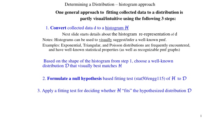
Determining a Distribution histogram approach One general approach to fitting collected data to a distribution is partly visual/intuitive using the following 3 steps: 1. Convert collected data d to a histogram H Next slide starts details about the histogram re-representation of d Notes: Histograms can be used to visually suggest/infer a well-known pmf. Examples: Exponential, Triangular, and Poisson distributions are frequently encountered, and have well-known statistical properties (as well as recognizable pmf graphs) Based on the shape of the histogram from step 1, choose a well-known distribution D that visually best matches H 2. Formulate a null hypothesis based fitting test (stat50/engg115) of H to D 3. Apply a fitting test for deciding whether H fits the hypothesized distribution D 1

Comparing Sample Histogram shapes (Source data unspecified) 1 of 3 A Ragged histogram 6 5 4 3 2 1 0 0 2 4 6 8 10 12 14 16 18 20 22 24 (Fig (1) Original Data - Too Ragged Alternating between histogram cells with 1) empty and 2) well-populated frequencies shape of section for large domain values (x < 4, and x > 12) unclear {most buckets have minimal population} 2

Comparing Sample Histogram shapes (Source data unspecified) 2 of 3 A Coarse histogram 25 20 15 10 5 0 0 ~ 7 8 ~ 15 16 ~ 24 (Fig (2) Combining adjacent cells - Too Coarse concentrated histogram cells with 1) zero frequency vs. 2) well-populated frequencies Overall shape unclear at a macro level, many different distributions look approximately like this 3

Comparing Sample Histogram shapes (Source data unspecified) 3 of 3 An appropriate histogram this histo shape is similar to a Poisson distribution with = 4 12 10 8 6 4 2 0 0~2 3~5 6~8 9~11 12~14 15~17 18~20 21~24 (Fig (3) Combining adjacent cells Appropriate each histogram cell (such as 0-5 or 6-15), etc. is well-populated ; entire histogram shape is evident; {all buckets in the range [0,24] have content, i.e., no empty buckets}; 4

Example Constructing a histogram from collected (aka raw) data The number of vehicles arriving at the northwest corner of a traffic intersection in a 5-minute period between 7:00 a.m. and 7:05 a.m. was monitored for the five workdays (Monday-Friday) over a 20-week period. The table (next slide) shows the collected data. This example from: Banks, Carson, Nelson and Nicol, Discrete-Event System Simulation , 4th Ed Data set d = one count value each workday for 20 weeks = 20*5 = 100 values (This data sample involves almost 8 times as many arrivals as the donut shop data) Each sample value is the count of vehicle arrivals at the intersection for one day, and these count values are the values of the rv of interest When d is represented as a frequency distribution table (next slide): The first entry (0,12) in the table indicates there were 12 5-minute periods during which no vehicles arrived; The second entry (1,10) indicates there were 10 5-minute periods during which one vehicle arrived; etc. The discrete random variable X in this scenario is: the number of vehicle arrivals in a 5-minute interval on a random workday The problem: determine the distribution D satisfied by the counts random variable. 5

Discrete Data Example (cont.) Arrivals per Period Frequency 0 1 2 3 4 5 Table Since X is a discrete variable, and since there is sufficient data, each histogram cell has Frequency >0 for each possible value in the range of data. Sufficient data (means: large-enough sample size) reveals relative probabilities more completely vs. lack of data (as illustrated in the Course Histogram (Fig(2)) The resulting histogram for the traffic data is shown in the next slide. Arrivals per Period 6 7 8 9 10 11 Frequency 7 5 5 3 3 1 12 10 19 17 10 8 6

Number of arrivals over 5-minute intervals - Discrete data example (cont.) 20 18 16 14 12 10 8 6 4 2 0 0 1 2 3 4 5 6 7 8 9 10 11 Histogram - Distribution of Number of arrivals per random time interval 7

Distribution Fitting Goodness-of-Fit Tests Two of the most common fit tests, with somewhat different approaches, are: a) Chi-Square test (partly visual, covered in this course) and b) Kolmogorov-Smirnov (aka KS) test (completely analytical/computational, not covered in CSC148): Any Fitting Test process evaluates a null hypotheses concerning whether a distribution of raw data fits a hypothesized distribution We will review the Null Hypothesis methodology soon Next = => the Chi-Square Goodness-of-Fit test for fitting a given distribution 8

Distribution Fitting, Chi-squared Fitting data to an assumed distribution: If d s histogram visually seems to follow a particular distribution (for example, the discrete Poisson), then choose that distribution family; next, select a specific pmf from Poisson family. Statistics obtained from d in your h3will determine the parameter of the ONE distribution family member as the candidate distribution pmf In summary, there are 2 major steps to Chi-squared fitting: 1. Determine appropriate distribution family F and Parameter(s) of F that determine one specific distribution candidate D (We say parameter(s) because each distribution Family has its own unique number (one or more) of parameters that differentiate family members 2. Doa Chi-squared statistical calculation & Null Hypothesis test on D and derive a fit decision 9

Chi-Square Test A Fitting Test evaluates how likely that the observation values (i.e., collected data) would be, assuming the null hypothesis is true. This test is valid for large sample sizes, for both discrete and continuous distributions when parameters are estimated by maximum likelihood. The test procedure begins by arranging n observations into k class intervals or cells. Then, calculate test statistic 2 i i 1 i = k = 2 0 --- (Eq 1) ( O E ) / E Oi the observed frequency of the ith class, and Ei expected frequency (computed using hypothesized distribution) of the ith class. Test basis: if Oi and Ei are close , ith summand of is a non-negative value that should be small => therefore, when each term is small, the sum must be relatively small for the data sample to fit the theoretical distribution i 2 0 2 0 Chi-Square has diverse applications (not just distribution fitting), such as: 1. Detecting a significant difference between observed Oi and expected Ei values 2. iid testing: if a sequence of random variable values are independent 3. computer security: whether decryption Dd of given encrypted data De succeeded 10

Goodness-of-Fit - Chi-Square Test (cont.) Given a Chi-Square test statistic for sample size n of random variable X. Next, define a null hypothesis and how to test its validity. The hypotheses are: H0:random variable X s values, conform to the distribution assumption with parameter(s) given by parameter estimate(s); this is the Null hypothesis. H1: random variable X, does not conform to the distribution 2 Critical values table Null hypothesis H0 is rejected if is found at many web sites (See Slide#22) 2 s k , 0 , k s 1 2 1 11

Goodness-of-Fit Tests - Chi-Square Test (cont.) Example: Chi-Square test applied to Poisson distribution Assumption In traffic example, the vehicle arrival data were analyzed. Since the histogram of the data (see Slide#7) seems to follow a Poisson distribution, parameter estimate, = 3.64 = x^ = mean of arrivals per observation is calculated by arithmetic mean: (total number of events (i.e. arrivals))/(total number of observations) (0*12 + 1*10 + 2*19 + 3*17 + 4*10 + + 1*11)/100 = 364/100 = 3.64 (Confirm the above calculation of frequency-formatted tabulation, Slide#6) The following hypotheses are formed: The random variable X whose distribution is to be tested is: number of vehicles arriving in the intersection in a given 5-minute interval on a workday H0: X is Poisson distributed with = frequency-weighted arrivals average H1: X is not Poisson distributed with the above mean 12

Goodness-of-Fit Tests Chi-Square Test (cont.) pmf for Poisson distribution of random variable x with mean is: (e- xi) / xi! , xi = 0, 1, 2 ... , 11 max observed arrivals count p(x=xi) is 0 , otherwise For = 3.64, the theoretical probabilities associated with various values of xi are obtained by the Eq 2 with the following results. Notice the twin peaks (adjacent almost equal values) p(0) = 0.026 p(3) = 0.211 p(6) = 0.085 p(1) = 0.096 p(4) = 0.192 p(7) = 0.044 p(2) = 0.174 p(5) = 0.140 p(8) = 0.020 (Eq 2) p(9) = 0.008 p(10) = 0.003 p(11) = 0.001 13

Chi-Square Test (cont.)RESUME traffic example - Combining classes 1) pi =prob(X=xi), so the predicted xi frequency in sample size n is: n*pi = 100*pi (because sample size is 100) Ei = n*pi; expected frequency of Ei also depends on sample size. TO EMPHASIZE: n = number of observations recorded/collected (=100) NOT total number of vehicles (=364) 2) Bracketed values combine >=2 classes into 1 class => How/Why are classes combined ? ==> Details on next slide. Expected Frequency, (Oi - Ei)2 / Ei n*pi=Ei (= ith test statistic term) 2.6 7.87 9.6 12.2 17.4 21.1 19.2 14.0 8.5 4.4 2.0 0.87.611.62 0.3 0.1 100.0 Observed Frequency, Oi xi 10 11 0 1 2 3 4 5 6 7 8 9 100 12 10 22 19 17 10 8 7 5 5 3 17 3 1 0.15 0.80 4.41 2.57 0.26 2 0 27.68 <- - Table CC Combining Classes: chi-squared goodness-of-fit test for traffic intersection example 14

Chi-Square Test (cont.) Guidelines for combining classes Given the results of the Ei calculations, Table CC was constructed. Review: Ej calculation is given for E1 (class#1, where p(0) = 0.026 ) Class#1 corresponds to the case of 0 arrivals in an observation Since the sample size n=100, E1 =np1= 100 (0.026) = 2.6, meaning the expected number of 5-minute intervals with 0 arrivals is 2.6. With mean 3.64, this seems sensible. In Chi-squared tests, if an Ei is quite small, the corresponding term of test statistic contributes a small value to the test statistic sum value, and several small Ei result in artificially-many classes Generally, practitioners use a minimum value of each Ej between 3 and 5, with 5 used very often ( There is both folklore and some science behind such recommended values, but there is no mathematical proof that dictates use of 5 or 4 or any exact preferred Ei value ) Thus, in Table CC, a) Since E1 = 2.6 < 5, E1 and E2 were combined. Since the original E1 + E2 = 2.6 + 9.6, the new combined class, renamed as E1, has value 12.2. b) By a) above, O1 and O2 are also combined, and k is reduced by one. c) In general, combining classes might need to be iterated over all adjacent classes; thus, the last five class intervals are all combined to become new class 7, and k is reduced by four more . . . The result is 7 classes, not the original 12 classes 15

python example: evaluating terms Ei of the Chi-Square fit - 1 of 2 """ chisquareCalcs_f22.py - CSC148 Poisson pmf & Chi-square Ei calculations Variable names uee terminolgy related to the Chi-square distribution fit """ import math # Built-in math module # User inputs numberOfClasses = int(input("Number of combined (if needed) Classes: ")) # Number of classes is type int OiFrequencyMean = float(input("Mean of the class frequencies: ")) # Mean derived from raw data sumOfxiFrequencies = int(input("sum of the class observations (= number of intervals measured): ")) # Observations count # The expected Poisson pmf pi values for above user-input parameters Poisson pmf evaluated at xi print("Chi-square class values calculations tool \n") print("The pmf values for pi = prob(X=xi), xi=0,1,2, ..., assuming NON-combined classes") for xi in range (numberOfClasses): print("p"+str(xi), " is: ",(math.exp(-OiFrequencyMean)*OiFrequencyMean**xi )/math.factorial(xi) ) print("") # The expected Ei values for the user-input parameters print(" \nThe Ei values for classes E1, E2, etc.") for xi in range (numberOfClasses): # xi ranges from 0 to (numberOfClasses-1) print("E"+str(xi), " is: ",sumOfxiFrequencies*(math.exp(-OiFrequencyMean)*OiFrequencyMean**xi )/math.factorial(xi)) Source file: chisquareCalcs_f23.py (Python3 calculation of ChiSquare test statistic terms Ei) = = > Execution results on next Slide 16

Python example: evaluating terms Ei of the Chi-Square fit 2 of 2 ============ RESTART: C:/Users/bill/148_f19/chisquareCalcs_s19.py ============ Number of Classes: 12 Mean of the class frequencies: 3.64 sum of the class frequencies: 100 Chi-Square class values calculations tool The pmf values for pi = prob(X=xi), xi=0,1,2, ..., using NON-combined classes p0 is: 0.02625234396568796 p1 is: 0.09555853203510419 p2 is: 0.17391652830388962 p3 is: 0.2110187210087194 p4 is: 0.19202703611793467 p5 is: 0.13979568229385644 p6 is: 0.08480938059160625 p7 is: 0.04410087790763525 p8 is: 0.02006589944797404 p9 is: 0.008115541554513944 Xi values 10 or larger produce very small Ei values p10 is: 0.0029540571258430764 p11 is: 0.0009775243580062542 The Ei values for classes E1, E2, etc. E0 is: 2.6252343965687963 E1 is: 9.555853203510418 E2 is: 17.391652830388963 E3 is: 21.10187210087194 E4 is: 19.202703611793467 E5 is: 13.979568229385645 E6 is: 8.480938059160625 E7 is: 4.410087790763526 E8 is: 2.006589944797404 E9 is: 0.8115541554513944 E10 is: 0.29540571258430764 E11 is: 0.09775243580062543 17

Chi-Square Test (cont.) Determining the Critical value Degrees of freedom terms: s= number of hypothesized distribution s parameters k = number of classes after combining classes 2 0 The calculated test statistic is 27.68 for the Traffic example The degrees of freedom (dof) for the tabulated value of 2is k-s-1 = 7-1-1 = 5 = . Here, s = 1, since Poisson distr. has 1 parameter. The -1 in (k s 1) is because when the test statistic value is known, then one of the terms in the test statistic sum is also determined. (dof is a measure of how many classes the test statistic involves) has thecritical value (rounded to 1 fractional digit)11.1 (see Table 4) At significance level 0.05, Ho is rejected. Specifically, we reject because there is only 5% probability (1 in 20) that a) our test statistic exceeds the critical value AND b) our data fits the distribution ==> The Traffic example analyst must now search for a better-fitting distribution Later in this module, consider What to do if a fit is unsuccessful 2 0 05 . , 5 18

homePage: ChiSquareDistributionFitVisualization.docx has additional background about the critical values table for distribution fitting P DF = 0.05 0.995 0.975 0.20 0.10 0.025 0.02 0.01 0.005 0.002 0.001 0.0000393 0.000982 1.642 2.706 3.841 5.024 5.412 6.635 7.879 9.550 10.828 1 0.0100 0.0506 3.219 4.605 5.991 7.378 7.824 9.210 10.597 12.429 13.816 2 0.0717 0.216 4.642 6.251 7.815 9.348 9.837 11.345 12.838 14.796 16.266 3 0.207 0.484 5.989 7.779 9.488 11.143 11.668 13.277 14.860 16.924 18.467 4 0.412 0.831 7.289 9.236 11.070 12.833 13.388 15.086 16.750 18.907 20.515 5 0.676 1.237 8.558 10.645 12.592 14.449 15.033 16.812 18.548 20.791 22.458 6 0.989 1.690 9.803 12.017 14.067 16.013 16.622 18.475 20.278 22.601 24.322 7 1.344 2.180 11.030 13.362 15.507 17.535 18.168 20.090 21.955 24.352 26.124 8 1.735 2.700 12.242 14.684 16.919 19.023 19.679 21.666 23.589 26.056 27.877 9 2.156 3.247 13.442 15.987 18.307 20.483 21.161 23.209 25.188 27.722 29.588 10 2.603 3.816 14.631 17.275 19.675 21.920 22.618 24.725 26.757 29.354 31.264 11 3.074 4.404 15.812 18.549 21.026 23.337 24.054 26.217 28.300 30.957 32.909 12 3.565 5.009 16.985 19.812 22.362 24.736 25.472 27.688 29.819 32.535 34.528 13 4.075 5.629 18.151 21.064 23.685 26.119 26.873 29.141 31.319 34.091 36.123 14 19 4.601 6.262 19.311 22.307 24.996 27.488 28.259 30.578 32.801 35.628 37.697 15

Outline of How test critical values are determined 1 of 2 Definitions Def A statistical hypothesis is a statement/assertion about a) the density function of a random variable rv OR b) more commonly, a property of a given density function (such as its mean, variance, etc.) This definition applies to both continuous and discrete rvs Def - a statistical hypothesis test is a procedure for deciding whether to accept/reject a given statistical hypothesis Note that a statistician (or simulation modeler involved with distributions of rvs) is free to design any test that is suitable for a given situation/study Hypothesis design; critical regions for a design for chi square Consider hypothesis design for specifying values of the fitting test statistic for which a statistical hypothesis H0 will be accepted. Although specific to the chi square statistic, the following design hypothesis discussion applies generally. 2 0 Def The chi square statistics values for rejecting H0 are (and historically have been) called the critical region of the test. Since the chi square statistics values are positive real numbers, a critical region is some subset of [y,+ ) of the positive real number axis. The non-critical region is then the complement of the critical region in (0,+ ) One of our goals is that of avoiding Type I error which means; rejecting H0 when it is actually true. The critical value corresponding to is the point y on the x-axis of the pdf for which *100 % of the area under the pdf lies to the right.The most common value is .05, although others such as .025 are used. For a specified , when > y, reject H0. With this inequality, Rejecting H0 will be incorrect only *100 % of the time. 0 20 2

Outline of How test critical values are determined 2 of 2 Theorem (used here but proven only in advanced statistics studies) The chi square statistic for k classes itself has a distribution approximated by a chi square distribution having (k-1) degrees of freedom. The theorem holds when the chi square statistic is calculated for arbitrarily many data collection sessions, not just one. Neither the traffic example, nor h3 involve a large number of chi square evaluations. Thus, our chi square fit process is approximate. Nonetheless, such an approximation is usually accurate enough for Poisson distribution fit for modeling an arrivals process. chi square distributions for various degrees of freedom (dof) values k21

chi square H0 decision for = 0.05 Each dof value corresponds to a different chi square distribution family member. Suppose that dof = 5 (the pdf in the family (not shown) is between Blue (dof=4) and Purple (dof=6) family members) The right-most 5% of the area under pdf for dof=5 has been tabulated in Table 4. The chi square value for dof=5 that determines the right-most 5% area under the corresponding pdf graph is 11.1 (= 11.07 rounded to a 1 digit of fraction). This 5% (considered as a probability) is the Ho hypothesis confidence level Any chi square test statistic that exceeds 11.1 is in the critical region for the chi square distribution having dof=5. There are several web sites (such as dunamath.com) with density and CDF calculators for various distributions. The chi square distribution is the specific gamma distribution with parameters k/2 and 2 ( parameterized by scale ), where k is the chi square dof ). f(x, ) denotes the gamma distribution (with customarily-named parameters and ) and the gamma function (x) as shown below. The critical values in Table 4 are obtained by working with these expressions. Summary: For rv x with pdf g(x), prob(y < x) = (% area under graph of g(x)) is given by evaluating CDF of g(x) = => For confidence level = .05, a chi square critical value x is obtained by solving (1 - .05) = CDF(x) for x. x can be found when the inverse function of the CDF(x) exists. Generally, x can only be solved by very complicated approximation mathematics when CDF(x) has no inverse. 22

A general Distribution Fitting algorithm - 1 of 2 Distribution-Fitting algorithm 1.Collect the raw data d 2.Convert a random variable s values in d to histogram representation H H Use H H to Suggest, and Choose a hypothesized D family 3.Identify parameter values for D D of step 2 (Example: if D is Poisson, find if exponential find etc.) 4.Test the decisions of steps 2 and 3 using a mathematically-based fitting test, such as Chi-square or Kolmogorov-Smirnov 5.IF fit was OK, use D and its identified parameters and EXIT ELSE (when D is apparently appropriate, but parameters wrong) OR (when D is determined to be incorrect) 23

A general distribution fitting algorithm - 2 of 2 The steps and embedded feedback in the Distribution-Fitting algorithm (previous slide) has advantages: 1. Repeatable technique regardless of the number of random processes identified in S that each need their distribution specified 2. Usable for either discrete or continuous hypothesized D D When the general distribution fitting algorithm fails Problem: Sometimes the search for identifying a suitable D fails. ? What to do ? Solution: Define a project/user-specific so-called empirical distribution. In this situation, the collected data d itself is used as the hypothesized distribution for the associated random variable. For example, in the traffic example earlier in this module, the table of (possible Xi value, fr is specified as the pmf for the random variable = (arrival counts in equal-sized small time intervals) { Of course, the DIS-advantage of an empirical distribution is that its CDF and any other distribution properties must be developed in DoItYourself (DIY) manner } 24