Average Parallelism and Speedup Performance Concepts

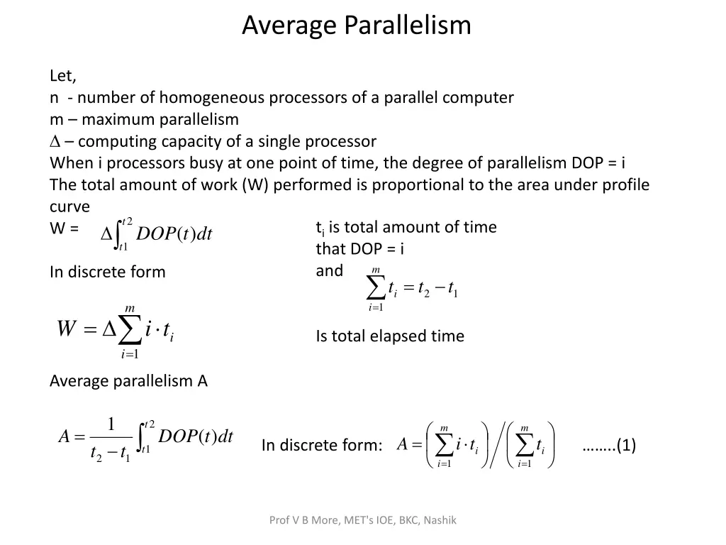
Average Parallelism Let, n - number of homogeneous processors of a parallel computer m maximum parallelism computing capacity of a single processor When i processors busy at one point of time, the degree of parallelism DOP = i The total amount of work (W) performed is proportional to the area under profile curve W = 1 t that DOP = i and 2 t ti is total amount of time ( ) DOP t dt m In discrete form = = t t t 2 1 i m 1 i = i = W i it Is total elapsed time 1 Average parallelism A 1 2 t m m = ( ) A DOP t dt = i = In discrete form: ..(1) = i 1 A i t t t t 1 t i i 2 1 1 Prof V B More, MET's IOE, BKC, Nashik

Speedup Performance Laws There are three speedup performance laws i) Amdahl s law based on fixed workload or fixed problem size ii) Gustafson s law applied to scaled problems where problem size increases with increase in machine size iii) Memory bound speedup model by Sun-Ni: scaled problems bounded by memory capacity Prof V B More, MET's IOE, BKC, Nashik

i) Amdahls law for a fixed workload - Real time response is demanded in many practical applications - computational workload is fixed with fixed problem size - Fixed load is shared among parallel processors for parallel execution to produce result as soon as possible, i.e. keeping turnaround time low. Asymptotic speedup S Speedup Sn = T1/Tn how much faster n processors compared to 1 processor m = m W i ) 1 ( T = = 1 i S . (2) ( ) T = i W i i 1 i is based on fixed workload regardless of machine size T(1) is execution time of workload on single processor T( ) is execution time of workload with infinite number of processors. Prof V B More, MET's IOE, BKC, Nashik

Fixed load speedup: Ideal speedup formula is described in equation (1) in previous slide. Consider both cases when DOP < n or DOP >= n When DOP = i > n , we assume all n processors are used to execute Wi exclusively. The execution time of Wi is ti(n) W i = ( ) i t n i i n Therefore response time is m W i = i = ( ) i T n i n 1 W = = ( ) ( ) i t n t When DOP = i < n, then i i i We can define fixed load speedup factor as ratio of T(1) to T( ) m = i W i T = = 1 1 i S T . (3) n + m W i Q = i + Q ( ) n ( ) n i n 1 Prof V B More, MET's IOE, BKC, Nashik Q(n) considered as lumpsum system overhead

We can now compare equation (1), (2), and (3) and say that Sn <= S <= A Amdahl s law implies that, sequential portion of program Wi does not change w.r.t. machine size n. whereas parallel portion is evenly executed by n processors. W1 + Wn = + (1- ) = 1 where is sequential portion and 1- is parallel portion. Is also called as Sequential Bottleneck, which can t be solved by increasing number of processors. Prof V B More, MET's IOE, BKC, Nashik

workload Execution time W1 W1 W1 W1 W1 W1 T1 T1 T1 T1 T1 Tn Wn Wn Wn Wn Wn Wn Tn T1 Tn Tn Tn Tn 1 2 3 4 5 6 n Number of processors 1 2 3 4 5 6 n Number of processors Fixed workload Decreasing execution time Sn 1024x S1024 = 1024 / (1+1023 ) Speedup 91x 1x 0% 100% Sequential fraction of program Speedup with a fixed load Prof V B More, MET's IOE, BKC, Nashik

ii) Gustafsons law of scaled problems Drawback of Amdahl s law is that the workload cannot be scaled to available computing power as machine size increases. Fixed load prevents scalability in performance. Gustafson proposed model that allows fixed-load problems to scaled speedup model. When resources are increased according to the need of high level of computational applications, it results very good and efficient resource utilization. Ex. Applications of weather forecasting 4 dimensional partial differential equation with very large number of grid points. When grid spacing is reduced, increases each dimension by factor of 10. Increases 104 times more grid points. Workload increases 10000 times. Fixed time speedup: Solves larger problems with increased load with same amount of time. Let, m - maximum DOP w.r.t. scaled problem. W i - scaled workload with DOP=i Prof V B More, MET's IOE, BKC, Nashik

In general, Wi > Wi for 2 <= i <= m and W1 = W1. The fixed time speedup is defined under the assumptions that, T(1) = T (1) (1) where T (1) is the execution time of the scaled problem and T(1) is the execution time of the original problem without scaling From above equation (1) we obtain W W i i = = ' ' m m i = + ( ) i Q n i i n 1 1 General formula for fixed time speedup is S n= T(1) / T (n) We obtain ' ' m m = ' = m ' ' W W i i = = ' 1 1 i i S n ' m i = i = i + ( ) W W Q n i i n 1 1 Prof V B More, MET's IOE, BKC, Nashik

workload Execution time W1 T1 T1 T1 T1 T1 T1 W1 W1 W1 W1 Wn Tn Tn Tn Tn Tn Tn Wn W1 Wn Wn Wn Wn 1 2 3 4 5 6 n 1 2 3 4 5 6 n Number of processors Number of processors Fixed Execution time Scaled Workload S n 1024x Sn = ( + n ( 1- ) ) / ( Speedup S 1024 = 1024 1023 1x 0% 100% Sequential fraction of program Speedup with a fixed execution time Prof V B More, MET's IOE, BKC, Nashik

Advantages: Gustafson s law support scalable performance as machine size increases. The problem can scale to match available computing power, Sequential fraction will not affect the performance as shown in figure. Prof V B More, MET's IOE, BKC, Nashik

iii) Memory-bounded speedup model (Sun, Ni) Large scale scientific / engineering computations requires larger memory. Local memory to each node is small. Node memory is collectively used according to the need of the parallel program. Fixed memory speedup: Let, M memory requirement of given problem W computational workload or M = g-1(W) W = g(M) two factors are bounded Memory capacity increases with increase in nodes in the system. = 1 i * m = W W is workload for sequential execution of program on single node. i * m = i is scaled workload for execution on n nodes, m* is maximum DOP of scaled problem = * * W W i 1 i m 1 g W Memory requirement for active node is bounded by i = 1 Prof V B More, MET's IOE, BKC, Nashik

Fixed memory speedup can be defined as * m = * W i = * n 1 i S * * m W i = i + ( ) Q n i i n 1 Wn= * * ( ) g nM The enhanced memory is related to scaled workload as: Where nM is increased memory capacity for n node multicomputer Assume, g*(nM) = G(n).Wn Wn* = G(n).Wn Where G(n) is the factor reflects increase in workload as memory increases n times. Fixed memory speedup can be re defined as + + * * ( ). W W W G ( n ). W = = * 1 1 + n n / S n * W W G n W n + * W n 1 n n 1 assuming Wi = 0 and Q(n) = 0 for simplicity Prof V B More, MET's IOE, BKC, Nashik

This fixed memory speedup model is valid under two assumptions: 1) Collection of all memory to form a global address space 2) All available memory areas are used for scaled problem. There are three special cases where the fixed memory speedup model can be applied: Case 1: G(n) = 1. Fixed memory speedup model becomes Amdahl s law when a fixed workload is given. Case 2: G(n) = n. Workload increases n times when memory increases n times. The model becomes Gustafson s law with fixed execution time. Case 3: G(n) > n. Computational workload increases faster than the memory requirement. The fixed memory model gives higher speedup than fixed time speedup. Amdahl s law and Gustafson s law are the special cases of fixed memory model. Prof V B More, MET's IOE, BKC, Nashik

workload Execution time T1 T1 T1 T1 T1 W1 T1 W1 W1 W1 W1 Wn Tn Tn Tn Tn Tn Tn Wn W1 Wn Wn Wn Wn 1 2 3 4 5 6 n 1 2 3 4 5 6 n Number of processors Number of processors Increased Execution time Scaled Workload Prof V B More, MET's IOE, BKC, Nashik