Basic Probability and Counting Rules Overview

Chapter 3 Basic Probability and Probability Distributions

Probability Terminology Classical Interpretation: Notion of probability based on equal likelihood of individual possibilities (coin toss has 1/2 chance of Heads, card draw has 4/52 chance of an Ace). Origins in games of chance. Outcome: Distinct result of random process (N= # outcomes) Event: Collection of outcomes (Ne= # of outcomes in event) Probability of event E: P(event E) = Ne/N Relative Frequency Interpretation: If an experiment were conducted repeatedly, what fraction of time would event of interest occur (based on empirical observation) Subjective Interpretation: Personal view (possibly based on external info) of how likely a one-shot experiment will end in event of interest

Obtaining Event Probabilities Classical Approach List all N possible outcomes of experiment List all Neoutcomes corresponding to event of interest (E) P(event E) = Ne/N Relative Frequency Approach Define event of interest Conduct experiment repeatedly (often using computer) Measure the fraction of time event E occurs Subjective Approach Obtain as much information on process as possible Consider different outcomes and their likelihood When possible, monitor your skill (e.g. stocks, weather)

Basic Counting Rules Multiplication Rule: Experiment has stages with possibilities at stage : k n i i k = Total possible outcomes: ... 1 2 n n n n k i = 1 i Example: Florida Lottery Pick 4 Game: At each stage, 10 possible numbers: Total: 10(10)(10)(10)=10,000 ( ) Permutations: Experiment involves selecting items from where order matters : k n k n ! n = n k + = n Total possible outcomes: ( 1)...( 1) P n n ( ) k ! n k Example: Selecting an executive c Total: 40(39)(38) = 59280 ommittee of 3 (President, Vice President, Treasurer) from 40 Member club: ( ) Combinations: Experiment involves selecting items from where order does not matter : k n k n n k n k + ( 1)...( 1) ! n n n = = = n k To tal possible outcomes: C ( ) ! ! ! k k n k Example: Florida Lotto: Commission 6 digits from 1:53 without replacement where order does not matter; 53! Total: 229574 80 7 = 6!4 !

Basic Probability and Rules A,B Events of interest P(A), P(B) Event probabilities Union: Event either A or B occurs (A B) Mutually Exclusive: A, B cannot occur together If A,B are mutually exclusive: P(either A or B) = P(A) + P(B) Complement of A: Event that A does not occur ( ) P( ) = 1- P(A) That is: P(A) + P( ) = 1 Intersection: Event both A and B occur (A B or AB) P (A B) = P(A) + P(B) - P(AB)

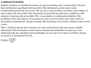
Conditional Probability and Independence Unconditional/Marginal Probability: Frequency which event occurs in general (given no additional info). P(A) Conditional Probability: Probability an event (A) occurs given knowledge another event (B) has occurred. P(A|B) Independent Events: Events whose unconditional and conditional (given the other) probabilities are the same ( ) ( ( | ) ( ) ( ) ( ) ( ( | ) ( ) ( ) ( ) ( ) ( ) ( | ) , independent ( ) A B P A = ) P A B P AB P B P AB P A P A P B A = = P A B P B ) P A B = = P B A P A P AB = = = ( ) ( | ) P B P A B P B P A B = ( | ) & ( ) P A B ( | ) P B A

John Snow London Cholera Death Study 2 Water Companies (Let D be the event of death): Southwark&Vauxhall (S): 264913 customers, 3702 deaths Lambeth (L): 171363 customers, 407 deaths Overall: 436276 customers, 4109 deaths 4109 = = ( ) 0094 . (94 per 10000 people) P D 436276 3702 = = ( | ) 0140 . (140 per 10000 people) P D S 264913 407 = = ( | ) 0024 . (24 per 10000 people) P D L 171363 Note that probability of death is almost 6 times higher for S&V customers than Lambeth customers (was important in showing how cholera spread)

John Snow London Cholera Death Study Cholera Death Water Company S&V Yes No Total 3702 (.0085) 407 (.0009) 4109 (.0094) 261211 (.5987) 170956 (.3919) 432167 (.9906) 264913 (.6072) 171363 (.3928) 436276 (1.0000) Lambeth Total ( Contingency Table with joint probabilities (in body of table) and marginal probabilities (on edge of table)

John Snow London Cholera Death Study Death Company .0140 D (.0085) S&V .6072 DC (.5987) .9860 WaterUser .0024 D (.0009) .3928 L DC (.3919) .9976 Tree Diagram obtaining joint probabilities by multiplication rule

Bayess Rule - Updating Probabilities Let A1, ,Ak be a set of events that partition a sample space such that (mutually exclusive and exhaustive): each set has known P(Ai) > 0 (each event can occur) for any 2 sets Ai and Aj, P(Aiand Aj) = 0 (events are disjoint) P(A1) + + P(Ak) = 1 (each outcome belongs to one of events) If C is an event such that 0 < P(C) < 1 (C can occur, but will not necessarily occur) We know the probability will occur given each event Ai: P(C|Ai) Then compute probability of Ai given C occurred: ( | ) ( P ) ( and C P ) P C A P + A P A C = = ( | ) i i i P A C i + ( | ) ( ) ( | ) ( ) ( ) P C A P A C A P A 1 1 k k

Northern Army at Gettysburg Regiment I Corps II Corps III Corps V Corps VI Corps XI Corps XII Corps Cav Corps Arty Reserve Sum Label A1 A2 A3 A4 A5 A6 A7 A8 A9 Initial # 10022 12884 11924 12509 15555 9839 8589 11501 2546 95369 Casualties 6059 4369 4211 2187 242 3801 1082 852 242 23045 P(Ai) 0.1051 0.1351 0.1250 0.1312 0.1631 0.1032 0.0901 0.1206 0.0267 1 P(C|Ai) 0.6046 0.3391 0.3532 0.1748 0.0156 0.3863 0.1260 0.0741 0.0951 P(C|Ai)*P(Ai) 0.0635 0.0458 0.0442 0.0229 0.0025 0.0399 0.0113 0.0089 0.0025 0.2416 P(C) P(Ai|C) 0.2630 0.1896 0.1828 0.0949 0.0105 0.1650 0.0470 0.0370 0.0105 1.0002 Regiments: partition of soldiers (A1, ,A9). Casualty: event C P(Ai) = (size of regiment) / (total soldiers) = (Column 3)/95369 P(C|Ai) = (# casualties) / (regiment size) = (Col 4)/(Col 3) P(C|Ai) P(Ai) = P(Ai and C) = (Col 5)*(Col 6) P(C)=sum(Col 7) P(Ai|C) = P(Ai and C) / P(C) = (Col 7)/.2416

Example - OJ Simpson Trial Given Information on Blood Test (T+/T-) Sensitivity: P(T+|Guilty)=1 Specificity: P(T-|Innocent)=.9957 P(T+|I)=.0043 Suppose you have a prior belief of guilt: P(G)=p* What is posterior probability of guilt after seeing evidence that blood matches: P(G|T+)? + + + + + = + = + = ( ) ( ) ( ) ( ) ( P G P T | ) ( ) ( P I P T | ) I P T = P T G + P T I G *(1) (1 *)(.0043) ) ( ) P T p p + + ( ( ) ( P G P T P T | ) *(1) p * P T G G p p + = = = = ( | ) P G T + + + + ( ) *(1) (1 *)(.0043) .9957 * .0043 p p Source: B.Forst (1996). Evidence, Probabilities and Legal Standards for Determination of Guilt: Beyond the OJ Trial , in Representing OJ: Murder, Criminal Justice, and the Mass Culture, ed. G. Barak pp. 22-28. Harrow and Heston, Guilderland, NY

Probability OJ is Guilty Given He Tested Positive 1 0.9 0.8 0.7 0.6 P(G|T+) 0.5 0.4 0.3 0.2 0.1 0 0 0.1 0.2 0.3 0.4 0.5 p* 0.6 0.7 0.8 0.9 1

Random Variables/Probability Distributions Random Variable: Outcome characteristic that is not known prior to experiment/observation Qualitative Variables: Characteristics that are non- numeric (e.g. gender, race, religion, severity) Quantitative Variables: Characteristics that are numeric (e.g. height, weight, distance) Discrete: Takes on only a countable set of possible values Continuous: Takes on values along a continuum Probability Distribution: Numeric description of outcomes of a random variable takes on, and their corresponding probabilities (discrete) or densities (continuous)

Discrete Random Variables Discrete RV: Can take on a finite (or countably infinite) set of possible outcomes Probability Distribution: List of values a random variable can take on and their corresponding probabilities Individual probabilities must lie between 0 and 1 Probabilities sum to 1 Notation: Random variable: Y Values Y can take on: y1, y2, , yk Probabilities: P(Y=y1) = p1 P(Y=yk) = pk p1+ + pk = 1

Example: Wars Begun by Year (1482-1939) Distribution of Numbers of wars started by year Y = # of wars started in randomly selected year Levels: y1=0, y2=1, y3=2, y4=3, y5=4 Probability Distribution: Histogram #Wars 0 1 2 3 4 Probability 0.5284 0.3231 0.1070 0.0328 0.0087 300 200 Yearr 100 0 0 1 2 3 4 More Wars

Masters Golf Tournament 1st Round Scores Score Frequency Probability 1 0.000288 2 0.000576 6 0.001728 16 0.004608 46 0.013249 67 0.019297 151 0.043491 238 0.068548 337 0.097062 428 0.123272 467 0.134505 498 0.143433 397 0.114343 293 0.084389 203 0.058468 125 0.036002 78 0.022465 50 0.014401 28 0.008065 17 0.004896 7 0.002016 7 0.002016 4 0.001152 3 0.000864 1 0.000288 2 0.000576 63 64 65 66 67 68 69 70 71 72 73 74 75 76 77 78 79 80 81 82 83 84 85 86 87 88 Histogram 600 500 Frequency 400 300 200 100 0 63 66 69 72 75 78 81 84 87 90 Score

Means and Variances of Random Variables Mean: Long-run averagea random variable will take on (also the balance point of the probability distribution) Expected Value is another term, however we really do not expect that a realization of X will necessarily be close to its mean. Notation: E{X} Variance: Average squared distance from the mean Mean and Variance of a discrete random variable: ( ) Y Y V Y E Y = = = = = + + + = E Y y p y p y p y p 1 1 2 2 Y k k i i ( ) 2 2 = 2 2 i 2 Y y p y p i Y i i = + 2 Y Standard Deviation (Same Units as Data): Y

Rules for Means Linear Transformations: a + bY (where a and b are constants): E{a+bY} = a+bY = a + b Y Sums of random variables: X + Y (where X and Y are random variables): E{X+Y} = X+Y = X + Y Linear Functions of Random Variables: E{a1Y1+ +anYn} = a 1+ +an n where E{Yi}= i

Example: Masters Golf Tournament Mean by Round (Note ordering): 1=73.54 2=73.07 3=73.76 4=73.91 Mean Score per hole (18) for round 1: E{(1/18)X1)}= (1/18) 1 = (1/18)73.54 = 4.09 Mean Score versus par (72) for round 1: E{X1-72} = X1-72 = 73.54-72= +1.54 (1.54 over par) Mean Difference (Round 1 - Round 4): E{X1-X4} = 1 - 4 = 73.54 - 73.91 = -0.37 Mean Total Score: E{X1+X2+X3+X4} = 1+ 2+ 3+ 4 = = 73.54+73.07+73.76+73.91 = 294.28 (6.28 over par)

Rules for Variances + = = 2 a bY 2 2 Y V a bY b + + = = + + 2 aX bY + 2 2 X 2 2 Y X 2 V aX bY a b ab X Y where is the correlation between and Y Special Cases: X and Y are independent (outcome of one does not alter the distribution of the other): = 0, last term drops out a=b=1 and = 0 V{X+Y} = X2 + Y2 a=1 b= -1 and = 0 V{X-Y} = X2 + Y2 a=b=1 and 0 V{X+Y} = X2 + Y2 + 2 X Y a=1 b= -1 and 0 V{X-Y} = X2 + Y2 -2 X Y

Examples - Wars & Masters Golf Score 63 64 65 66 67 68 69 70 71 72 73 74 75 76 77 78 79 80 81 82 83 84 85 86 87 88 Sum prob 0.000288 0.000576 0.001728 0.004608 0.013249 0.019297 0.043491 0.068548 0.097062 0.123272 0.134505 0.143433 0.114343 0.084389 0.058468 0.036002 0.022465 0.014401 0.008065 0.004896 0.002016 0.002016 0.001152 0.000864 0.000288 0.000576 1 x*p 0.0181 0.0369 0.1123 0.3041 0.8877 1.3122 3.0009 4.7984 6.8914 8.8756 9.8188 10.6141 8.5757 6.4136 4.5020 2.8082 1.7748 1.1521 0.6532 0.4015 0.1673 0.1694 0.0979 0.0743 0.0251 0.0507 73.54 #Wars 0 1 2 3 4 Sum Probability 0.5284 0.3231 0.1070 0.0328 0.0087 1.0000 x*p 0.0000 0.3231 0.2140 0.0983 0.0349 0.6703 =0.67 =73.54

Binomial Distribution for Sample Counts Binomial Experiment Consists of n trials or observations Trials/observations are independent of one another Each trial/observation can end in one of two possible outcomes often labelled Success and Failure The probability of success, , is constant across trials/observations Random variable, Y, is the number of successes observed in the n trials/observations. Binomial Distributions: Family of distributions for Y, indexed by Success probability ( ) and number of trials/observations (n). Notation: Y~Bin(n, )

Binomial Distributions and Sampling To obtain the probability of observing y successes in the n trials, there are two components: The number of possible arrangements of the y successes and the n-y failures among the n trials The probability of each of those arrangements = n y ! n = Number of possible arrangements: 0,1, , y n !( )! y n y n y y Probability of each arrangement: (1 ) n y n y = = = y ( ) ( ) (1 ) P Y y P y

Example - Diagnostic Test Test claims to have a sensitivity of 90% (Among people with condition, probability of testing positive is .90) 10 people who are known to have condition are identified, Y is the number that correctly test positive 5 10 y 10 y 10! ( ) = = = = 10 y y (.9) (.1) 0,1, ,10 P Y y y ( ) ! 10 ! y y y P(y) 0 1 2 3 4 6 7 8 9 10 1E-10 9E-09 3.64E-07 8.75E-06 0.000138 0.001488 0.01116 0.057396 0.19371 0.38742 0.348678 Table can be obtained in R with function: dbinom(0:10,10,0.9) pth Quantile in R (0 < p < 1): qbinom(p, n, ) P(Y y) in R: P(y) in R: pbinom(y, n, ) dbinom(y, n, )

Binomial Mean & Standard Deviation Let Si=1 if the ith trial was a success, 0 otherwise Then P(Si=1) = and P(Si=0) = 1- Then E{Si}= S = 1( ) + 0(1- ) = Note that Y = S1+ +Sn and that trials are independent Then E{Y}= Y = n S = n V{Si} = E{Si2}- S2 = - 2 = (1- ) Then V{Y}= Y2 =n (1- ) E Y ( , ) = = = ~ (1 ) Y Bin n n n Y Y = 0 . 9 = = = For the diagnostic test : ) 9 . 0 ( 10 9 . 0 ( 10 ) 1 . 0 )( . 0 95

Poisson Distribution for Event Counts Distribution related to Binomial for Counts of number of events occurring in fixed time or space. Takes many sub-intervals and assumes Binomial (n=1) distribution for events in each. The average number of events in unit time or space is . In general, for length t, mean is t y i e y x i ( ) ( ) = = = = = x 0,1,2,.... 2.71828 P Y y P y y e e ! ! = 0 i pth Quantile in R (0 < p < 1): qpois(p, ) P(Y y) in R: ppois(y, ) P(y) in R: dpois(y, )

Poisson Distribution for Event Counts y i e y x i ( ) ( ) = = = = = x 0,1,2,.... 2.71828 P Y y P y y e e ! ! = 0 i 1 y y y y e y e y e e E Y = = = = = y y ( ) ( ) ! ! 1 ! 1 ! y y = = = = 0 1 1 1 y y y y 1 y = = e e = e ( ) 1 ! y = 1 y 2 y y y e y e y e e ( ) ( ) ( ) = = = = = 2 1 1 1 E Y Y y y y y ( ) ( ) ! ! 2 ! 2 ! y y = = = = 0 2 2 2 y y y y 2 y = = = 2 2 2 e e e ( ) 2 ! y = 2 y E Y ( ) E Y E Y = + = + 2 2 1 E Y Y E Y 2 2 = = = + = 2 2 2 V Y

Continuous Random Variables Variable can take on any value along a continuous range of numbers (interval) Probability distribution is described by a smooth density curve Probabilities of ranges of values for Y correspond to areas under the density curve Curve must lie on or above the horizontal axis Total area under the curve is 1 Special cases: Normal and Gamma distributions

Normal Distribution Bell-shaped, symmetric family of distributions Classified by 2 parameters: Mean ( ) and standard deviation ( ). These represent location and spread Random variables that are approximately normal have the following properties wrt individual measurements: Approximately half (50%) fall above (and below) mean Approximately 68% fall within 1 standard deviation of mean Approximately 95% fall within 2 standard deviations of mean Virtually all fall within 3 standard deviations of mean Notation when Y is normally distributed with mean and standard deviation : Y ~ N( ) ( )2 2 y ( ) ( f y ) 1/2 = 2 Density function 2 , , 0 e y 2

Two Normal Distributions Note: IQ scores follow the lower Normal Distribution ( =100, =15)

Normal Distribution = + + ( ) . 0 50 ( ) . 0 68 ( 2 2 ) . 0 95 P Y P Y P Y

Standard Normal (Z) Distribution Problem: Unlimited number of possible normal distributions (- < < , > 0) Solution: Standardize the random variable to have mean 0 and standard deviation 1 Y = ~ ( , ) ~ ) 1 , 0 ( N Y N Z Probabilities of certain ranges of values and specific percentiles of interest can be obtained through the standard normal (Z) distribution

2nd decimal place z 0.00 0.5000 0.4602 0.4207 0.3821 0.3446 0.3085 0.2743 0.2420 0.2119 0.1841 0.1587 0.1357 0.1151 0.0968 0.0808 0.0668 0.0548 0.0446 0.0359 0.0287 0.0228 0.0179 0.0139 0.0107 0.0082 0.0062 0.0047 0.0035 0.0026 0.0019 0.01 0.4960 0.4562 0.4168 0.3783 0.3409 0.3050 0.2709 0.2389 0.2090 0.1814 0.1562 0.1335 0.1131 0.0951 0.0793 0.0655 0.0537 0.0436 0.0351 0.0281 0.0222 0.0174 0.0136 0.0104 0.0080 0.0060 0.0045 0.0034 0.0025 0.0018 0.02 0.4920 0.4522 0.4129 0.3745 0.3372 0.3015 0.2676 0.2358 0.2061 0.1788 0.1539 0.1314 0.1112 0.0934 0.0778 0.0643 0.0526 0.0427 0.0344 0.0274 0.0217 0.0170 0.0132 0.0102 0.0078 0.0059 0.0044 0.0033 0.0024 0.0018 0.03 0.4880 0.4483 0.4090 0.3707 0.3336 0.2981 0.2643 0.2327 0.2033 0.1762 0.1515 0.1292 0.1093 0.0918 0.0764 0.0630 0.0516 0.0418 0.0336 0.0268 0.0212 0.0166 0.0129 0.0099 0.0075 0.0057 0.0043 0.0032 0.0023 0.0017 0.04 0.4840 0.4443 0.4052 0.3669 0.3300 0.2946 0.2611 0.2296 0.2005 0.1736 0.1492 0.1271 0.1075 0.0901 0.0749 0.0618 0.0505 0.0409 0.0329 0.0262 0.0207 0.0162 0.0125 0.0096 0.0073 0.0055 0.0041 0.0031 0.0023 0.0016 0.05 0.4801 0.4404 0.4013 0.3632 0.3264 0.2912 0.2578 0.2266 0.1977 0.1711 0.1469 0.1251 0.1056 0.0885 0.0735 0.0606 0.0495 0.0401 0.0322 0.0256 0.0202 0.0158 0.0122 0.0094 0.0071 0.0054 0.0040 0.0030 0.0022 0.0016 0.06 0.4761 0.4364 0.3974 0.3594 0.3228 0.2877 0.2546 0.2236 0.1949 0.1685 0.1446 0.1230 0.1038 0.0869 0.0721 0.0594 0.0485 0.0392 0.0314 0.0250 0.0197 0.0154 0.0119 0.0091 0.0069 0.0052 0.0039 0.0029 0.0021 0.0015 0.07 0.4721 0.4325 0.3936 0.3557 0.3192 0.2843 0.2514 0.2206 0.1922 0.1660 0.1423 0.1210 0.1020 0.0853 0.0708 0.0582 0.0475 0.0384 0.0307 0.0244 0.0192 0.0150 0.0116 0.0089 0.0068 0.0051 0.0038 0.0028 0.0021 0.0015 0.08 0.4681 0.4286 0.3897 0.3520 0.3156 0.2810 0.2483 0.2177 0.1894 0.1635 0.1401 0.1190 0.1003 0.0838 0.0694 0.0571 0.0465 0.0375 0.0301 0.0239 0.0188 0.0146 0.0113 0.0087 0.0066 0.0049 0.0037 0.0027 0.0020 0.0014 0.09 0.4641 0.4247 0.3859 0.3483 0.3121 0.2776 0.2451 0.2148 0.1867 0.1611 0.1379 0.1170 0.0985 0.0823 0.0681 0.0559 0.0455 0.0367 0.0294 0.0233 0.0183 0.0143 0.0110 0.0084 0.0064 0.0048 0.0036 0.0026 0.0019 0.0014 I n t e g e r p a r t & 1 s 0.0 0.1 0.2 0.3 0.4 0.5 0.6 0.7 0.8 0.9 1.0 1.1 1.2 1.3 1.4 1.5 1.6 1.7 1.8 1.9 2.0 2.1 2.2 2.3 2.4 2.5 2.6 2.7 2.8 2.9 t d e c i m a l Upper tail probabilities (symmetric distribution)

Finding Probabilities of Specific Ranges Step 1 - Identify the normal distribution of interest (e.g. its mean ( ) and standard deviation ( ) ) Step 2 - Identify the range of values that you wish to determine the probability of observing (yL , yU), where often the upper or lower bounds are or - Step 3 - Transform yL and yU into Z-values: y y = = U L z z L U Step 4 - Obtain P(zL Z zU) from Z-table

Example IQ Scores What is the probability a randomly selected person has an IQ score of 120 or above? Step 1 -Y ~ N(100 , 15) Step 2 -yL = 120.0 yU = Step 3 - 120 100 15 = = = 1.33 z z L U Step 4 - P(Y 120) = P(Z 1.33) = .0918 z 0.02 0.1112 0.0934 0.0778 0.03 0.1093 0.0918 0.0764 0.04 0.1075 0.0901 0.0749 1.2 1.3 1.4

Finding Percentiles of a Distribution Step 1 - Identify the normal distribution of interest (e.g. its mean ( ) and standard deviation ( ) ) Step 2- Determine the percentile of interest 100p% (e.g. the 90th percentile is the cut-off where only 90% of scores are below and 10% are above). Step 3 - Find 1-p in the body of the z-table and its corresponding z-value (z1-p) on the outer edge: If 100p 50 then look for z1-p corresponding to upper area 1-p If 100p < 50 then take the negative value z1-p=-zp Step 4 - Transform zp back to original units: y = + z 1 p p

Example IQ Scores Above what IQ Score do the highest 5% lie above? Step 1 - Y ~ N(100 , 15) Step 2 - Want to determine 95th percentile (p = .95, 1-p = .05) Step 3 - P(Z 1.645) = .05 Step 4 - y.95 = 100 + (1.645)(15) = 100 + 24.675 = 124.675 Note that the 5th percentile is 100 24.675 = 75.325 z 0.03 0.0630 0.0516 0.0418 0.04 0.0618 0.0505 0.0409 0.05 0.0606 0.0495 0.0401 0.06 0.0594 0.0485 0.0392 1.5 1.6 1.7 pth Quantile in R (0 < p < 1): qnorm(p , ) P(Y y) in R: pnorm(y, ) Density f(y) in R: dnorm(y, )

Assessing Normality and R Functions Obtain a histogram and see if mound-shaped Obtain a normal probability plot Order data from smallest to largest and rank them (1 to n) Obtain a quantile for each: q = (rank-0. 5) / n Obtain the z-score corresponding to the quantile Plot observed data versus z-score, see if straight line (approx.) R Commands: qqnorm(y); qqline(y) The Shapiro-Wilk Test can be run, with the null hypothesis being that the measurements are normally distributed. In R: shapiro.test(y)

Chi-Square Distribution Indexed by degrees of freedom ( ) X~ Z~N(0,1) Z2 ~ Assuming Independence: n = 2 2 ,..., ~ 1,..., ~ X X i n X 1 n i i i = 1 i Density Function: 1 ( ) f x ( ) 2 1 = 2 x 0, 0 x e x 2 2 2 pth Quantile in R (0 < p < 1): qchisq(p , ) P(X x) in R: pchisq(x, ) Density f(x) in R: dchisq(x, )

Chi-Square Distributions Chi-Square Distributions 0.2 0.18 df=4 0.16 df=10 0.14 df=20 0.12 f1(y) f2(y) f3(y) f4(y) f5(y) df=30 f(X^2) 0.1 df=50 0.08 0.06 0.04 0.02 0 0 10 20 30 40 50 60 70 X^2

Critical Values for Chi-Square Distributions (Upper Tail Probabilities) df\F(x) 1 2 3 4 5 6 7 8 9 10 11 12 13 14 15 16 17 18 19 20 21 22 23 24 25 26 27 28 29 30 40 50 60 70 80 90 100 0.995 0.000 0.010 0.072 0.207 0.412 0.676 0.989 1.344 1.735 2.156 2.603 3.074 3.565 4.075 4.601 5.142 5.697 6.265 6.844 7.434 8.034 8.643 9.260 9.886 10.520 11.160 11.808 12.461 13.121 13.787 20.707 27.991 35.534 43.275 51.172 59.196 67.328 0.99 0.000 0.020 0.115 0.297 0.554 0.872 1.239 1.646 2.088 2.558 3.053 3.571 4.107 4.660 5.229 5.812 6.408 7.015 7.633 8.260 8.897 9.542 10.196 10.856 11.524 12.198 12.879 13.565 14.256 14.953 22.164 29.707 37.485 45.442 53.540 61.754 70.065 0.975 0.001 0.051 0.216 0.484 0.831 1.237 1.690 2.180 2.700 3.247 3.816 4.404 5.009 5.629 6.262 6.908 7.564 8.231 8.907 9.591 10.283 10.982 11.689 12.401 13.120 13.844 14.573 15.308 16.047 16.791 24.433 32.357 40.482 48.758 57.153 65.647 74.222 0.95 0.004 0.103 0.352 0.711 1.145 1.635 2.167 2.733 3.325 3.940 4.575 5.226 5.892 6.571 7.261 7.962 8.672 9.390 10.117 10.851 11.591 12.338 13.091 13.848 14.611 15.379 16.151 16.928 17.708 18.493 26.509 34.764 43.188 51.739 60.391 69.126 77.929 0.9 0.016 0.211 0.584 1.064 1.610 2.204 2.833 3.490 4.168 4.865 5.578 6.304 7.042 7.790 8.547 9.312 10.085 10.865 11.651 12.443 13.240 14.041 14.848 15.659 16.473 17.292 18.114 18.939 19.768 20.599 29.051 37.689 46.459 55.329 64.278 73.291 82.358 0.1 2.706 4.605 6.251 7.779 9.236 10.645 12.017 13.362 14.684 15.987 17.275 18.549 19.812 21.064 22.307 23.542 24.769 25.989 27.204 28.412 29.615 30.813 32.007 33.196 34.382 35.563 36.741 37.916 39.087 40.256 51.805 63.167 74.397 85.527 96.578 107.565 118.498 0.05 3.841 5.991 7.815 9.488 11.070 12.592 14.067 15.507 16.919 18.307 19.675 21.026 22.362 23.685 24.996 26.296 27.587 28.869 30.144 31.410 32.671 33.924 35.172 36.415 37.652 38.885 40.113 41.337 42.557 43.773 55.758 67.505 79.082 90.531 101.879 113.145 124.342 0.025 5.024 7.378 9.348 11.143 12.833 14.449 16.013 17.535 19.023 20.483 21.920 23.337 24.736 26.119 27.488 28.845 30.191 31.526 32.852 34.170 35.479 36.781 38.076 39.364 40.646 41.923 43.195 44.461 45.722 46.979 59.342 71.420 83.298 95.023 106.629 118.136 129.561 0.01 6.635 9.210 11.345 13.277 15.086 16.812 18.475 20.090 21.666 23.209 24.725 26.217 27.688 29.141 30.578 32.000 33.409 34.805 36.191 37.566 38.932 40.289 41.638 42.980 44.314 45.642 46.963 48.278 49.588 50.892 63.691 76.154 88.379 100.425 112.329 124.116 135.807 0.005 7.879 10.597 12.838 14.860 16.750 18.548 20.278 21.955 23.589 25.188 26.757 28.300 29.819 31.319 32.801 34.267 35.718 37.156 38.582 39.997 41.401 42.796 44.181 45.559 46.928 48.290 49.645 50.993 52.336 53.672 66.766 79.490 91.952 104.215 116.321 128.299 140.169

Students t-Distribution Indexed by degrees of freedom ( ) X~t Z~N(0,1), X~ Assuming Independence of Z and X: Z X = ~ T t Density Function: + 1 + 1 2 t 2 2 ( ) = + 1 0 f t t 2 pth Quantile in R (0 < p < 1): qt(p , ) P(T t) in R: pt(t, ) Density f(t) in R: dt(t, )

t(3), t(11), t(24), Z Distributions 0.45 0.4 0.35 0.3 0.25 f(t_3) 0.2 Density f(t_11) f(t_24) 0.15 Z~N(0,1) 0.1 0.05 0 -3 -2 -1 0 1 2 3 t (z)

Critical Values for Students t-Distributions (Upper Tail Probabilities) df\F(t) 1 2 3 4 5 6 7 8 9 10 11 12 13 14 15 16 17 18 19 20 21 22 23 24 25 26 27 28 29 30 40 50 60 70 80 90 100 0.1 3.078 1.886 1.638 1.533 1.476 1.440 1.415 1.397 1.383 1.372 1.363 1.356 1.350 1.345 1.341 1.337 1.333 1.330 1.328 1.325 1.323 1.321 1.319 1.318 1.316 1.315 1.314 1.313 1.311 1.310 1.303 1.299 1.296 1.294 1.292 1.291 1.290 0.05 6.314 2.920 2.353 2.132 2.015 1.943 1.895 1.860 1.833 1.812 1.796 1.782 1.771 1.761 1.753 1.746 1.740 1.734 1.729 1.725 1.721 1.717 1.714 1.711 1.708 1.706 1.703 1.701 1.699 1.697 1.684 1.676 1.671 1.667 1.664 1.662 1.660 0.025 12.706 4.303 3.182 2.776 2.571 2.447 2.365 2.306 2.262 2.228 2.201 2.179 2.160 2.145 2.131 2.120 2.110 2.101 2.093 2.086 2.080 2.074 2.069 2.064 2.060 2.056 2.052 2.048 2.045 2.042 2.021 2.009 2.000 1.994 1.990 1.987 1.984 0.01 31.821 6.965 4.541 3.747 3.365 3.143 2.998 2.896 2.821 2.764 2.718 2.681 2.650 2.624 2.602 2.583 2.567 2.552 2.539 2.528 2.518 2.508 2.500 2.492 2.485 2.479 2.473 2.467 2.462 2.457 2.423 2.403 2.390 2.381 2.374 2.368 2.364 0.005 63.657 9.925 5.841 4.604 4.032 3.707 3.499 3.355 3.250 3.169 3.106 3.055 3.012 2.977 2.947 2.921 2.898 2.878 2.861 2.845 2.831 2.819 2.807 2.797 2.787 2.779 2.771 2.763 2.756 2.750 2.704 2.678 2.660 2.648 2.639 2.632 2.626

F-Distribution Indexed by 2 degrees of freedom ( ) W~F X1 ~ , X2 ~ Assuming Independence of X1 and X2: X X = ~ 1 1 W F , 1 2 2 2 Density Function: + + 1 2 + 1 1 2 1 2 1 1 2 w 2 2 2 1 2 1 ( ) f w = + 1 0 , 0 1 1 w w 2 1 2 + 1 2 1 2 2 2 2 2 2 2 pth Quantile in R (0 < p < 1): qf(p , ) P(W w) in R: pf(w, ) Density f(w) in R: df(w, )

F-Distributions 0.9 0.8 0.7 0.6 Density Function of F 0.5 f(5,5) 0.4 f(5,10) f(10,20) 0.3 0.2 0.1 0 0 1 2 3 4 5 6 7 8 9 10 -0.1 F

Critical Values for F-distributions P(F Table Value) = 0.05 df2\df1 1 2 3 4 5 6 7 8 9 10 11 12 13 14 15 16 17 18 19 20 21 22 23 24 25 26 27 28 29 30 40 50 60 70 80 90 100 1 2 3 4 5 6 7 8 9 10 161.45 18.51 10.13 7.71 6.61 5.99 5.59 5.32 5.12 4.96 4.84 4.75 4.67 4.60 4.54 4.49 4.45 4.41 4.38 4.35 4.32 4.30 4.28 4.26 4.24 4.23 4.21 4.20 4.18 4.17 4.08 4.03 4.00 3.98 3.96 3.95 3.94 199.50 19.00 9.55 6.94 5.79 5.14 4.74 4.46 4.26 4.10 3.98 3.89 3.81 3.74 3.68 3.63 3.59 3.55 3.52 3.49 3.47 3.44 3.42 3.40 3.39 3.37 3.35 3.34 3.33 3.32 3.23 3.18 3.15 3.13 3.11 3.10 3.09 215.71 19.16 9.28 6.59 5.41 4.76 4.35 4.07 3.86 3.71 3.59 3.49 3.41 3.34 3.29 3.24 3.20 3.16 3.13 3.10 3.07 3.05 3.03 3.01 2.99 2.98 2.96 2.95 2.93 2.92 2.84 2.79 2.76 2.74 2.72 2.71 2.70 224.58 19.25 9.12 6.39 5.19 4.53 4.12 3.84 3.63 3.48 3.36 3.26 3.18 3.11 3.06 3.01 2.96 2.93 2.90 2.87 2.84 2.82 2.80 2.78 2.76 2.74 2.73 2.71 2.70 2.69 2.61 2.56 2.53 2.50 2.49 2.47 2.46 230.16 19.30 9.01 6.26 5.05 4.39 3.97 3.69 3.48 3.33 3.20 3.11 3.03 2.96 2.90 2.85 2.81 2.77 2.74 2.71 2.68 2.66 2.64 2.62 2.60 2.59 2.57 2.56 2.55 2.53 2.45 2.40 2.37 2.35 2.33 2.32 2.31 233.99 19.33 8.94 6.16 4.95 4.28 3.87 3.58 3.37 3.22 3.09 3.00 2.92 2.85 2.79 2.74 2.70 2.66 2.63 2.60 2.57 2.55 2.53 2.51 2.49 2.47 2.46 2.45 2.43 2.42 2.34 2.29 2.25 2.23 2.21 2.20 2.19 236.77 19.35 8.89 6.09 4.88 4.21 3.79 3.50 3.29 3.14 3.01 2.91 2.83 2.76 2.71 2.66 2.61 2.58 2.54 2.51 2.49 2.46 2.44 2.42 2.40 2.39 2.37 2.36 2.35 2.33 2.25 2.20 2.17 2.14 2.13 2.11 2.10 238.88 19.37 8.85 6.04 4.82 4.15 3.73 3.44 3.23 3.07 2.95 2.85 2.77 2.70 2.64 2.59 2.55 2.51 2.48 2.45 2.42 2.40 2.37 2.36 2.34 2.32 2.31 2.29 2.28 2.27 2.18 2.13 2.10 2.07 2.06 2.04 2.03 240.54 19.38 8.81 6.00 4.77 4.10 3.68 3.39 3.18 3.02 2.90 2.80 2.71 2.65 2.59 2.54 2.49 2.46 2.42 2.39 2.37 2.34 2.32 2.30 2.28 2.27 2.25 2.24 2.22 2.21 2.12 2.07 2.04 2.02 2.00 1.99 1.97 241.88 19.40 8.79 5.96 4.74 4.06 3.64 3.35 3.14 2.98 2.85 2.75 2.67 2.60 2.54 2.49 2.45 2.41 2.38 2.35 2.32 2.30 2.27 2.25 2.24 2.22 2.20 2.19 2.18 2.16 2.08 2.03 1.99 1.97 1.95 1.94 1.93

Sampling Distributions Distribution of a Sample Statistic: The probability distribution of a sample statistic obtained from a random sample or a randomized experiment What values can a sample mean (or proportion) take on and how likely are ranges of values? Population Distribution: Set of values for a variable for a population of individuals. Conceptually equivalent to probability distribution in sense of selecting an individual at random and observing their value of the variable of interest