Bayes for Beginners
The content discusses a scenario where a diagnostic test is used to determine the probability of an individual having a disease. It delves into Bayesian probability calculations to ascertain the likelihood of disease presence given a positive test result. Through detailed explanations and equations, the concept of prior probabilities, likelihood, and marginal probabilities is explored to understand how the test result affects the overall probability of disease occurrence.

Download Presentation

Please find below an Image/Link to download the presentation.
The content on the website is provided AS IS for your information and personal use only. It may not be sold, licensed, or shared on other websites without obtaining consent from the author.If you encounter any issues during the download, it is possible that the publisher has removed the file from their server.
You are allowed to download the files provided on this website for personal or commercial use, subject to the condition that they are used lawfully. All files are the property of their respective owners.
The content on the website is provided AS IS for your information and personal use only. It may not be sold, licensed, or shared on other websites without obtaining consent from the author.
E N D
Presentation Transcript
Bayes for Beginners Rumana Chowdhury & Peter Smittenaar Methods for Dummies 2011 Dec 7th 2011
A disease occurs in 0.5% of population A diagnostic test gives a positive result in 99% of people that have the disease in 5% of people that do not have the disease (false positive) A random person from the street is found to be positive on this test. What is the probability that they have the disease? A: 0-30% B: 30-60% C: 60-90%
A disease occurs in 0.5% of population A diagnostic test gives a positive result in 99% of people that have the disease in 5% of people that do not have the disease (false positive) A = disease B = positive test result P(A) = 0.005 P(~A) = 1 0.005 = 0.995 P(B) = 0.005 * 0.99 (people with disease) + 0.995 * 0.05 (people without disease) = 0.0547 (slightly more than 5% of all tests are positive) probability of having disease probability of not having disease conditional probabilities P(B|A) = 0.99 P(~B|A) = 1 0.99 = 0.01 P(B|~A) = 0.05 P(~B|~A) = 1 0.05 = 0.95 probability of pos result given you have disease probability of neg result given you have disease probability of pos result given you do not have disease probability of neg result given you do not have disease P(A|B) is probability of disease given the test is positive (which is what we re interested in) Very different from P(B|A): probability of positive test results given you have the disease.
A = disease B = positive test result population = 100 positive test result P(B) 5.47 disease P(A) 0.5
A = disease B = positive test result population = 100 P(A,B) is the joint probability, or the probability that both events occur. P(A,B) is the same as P(B,A). But we already know that the test was positive, so we have to take that into account. Of all the people already in the green circle, how many fall into the P(A,B) part? That s the probability we want to know! positive test result P(B) 5.47 That is: P(A|B) = P(A,B) / P(B) P(B,~A) You can write down same thing for the inverse: P(B|A) = P(A,B) / P(A) disease P(A) 0.5 P(A,B) The joint probability can be expressed in two ways by rewriting the equations P(A,B) = P(A|B) * P(B) P(A,B) = P(B|A) * P(A) Equating the two gives P(A|B) * P(B) = P(B|A) * P(A) P(A,~B) P(A|B) = P(B|A) * P(A) / P(B)
A = disease B = positive test result P(A) = 0.005 P(B|A) = 0.99 P(B) = 0.005 * 0.99 (people with disease) + 0.995 * 0.05 (people without disease) = 0.0547 probability of having disease probability of pos result given you have disease Bayes Theorem P(A|B) = P(B|A) * P(A) / P(B) P(A|B) = 0.99 * 0.005 / 0.0547 = 0.09 So a positive test result increases your probability of having the disease to only 9%, simply because the disease is very rare (relative to the false positive rate). P(A) is called the prior: before we have any information, we estimate the chance of having the disease 0.5% P(B|A) is called the likelihood: probability of the data (pos test result) given an underlying cause (disease) P(B) is the marginal probability of the data: the probability of observing this particular outcome, taken over all possible values of A (disease and no disease) P(A|B) is the posteriorprobability: it is a combination of what you thought before obtaining the data, and the new information the data provided (combination of prior and likelihood)
Lets do another one It rains on 20% of days. When it rains, it was forecasted 80% of the time When it doesn t rain, it was erroneously forecasted 10% of the time. The weatherman forecasts rain. What s the probability of it actually raining? A = forecast rain B = it rains What information is given in the story? P(B) = 0.2 (prior) P(A|B) = 0.8 (likelihood) P(A|~B) = 0.1 P(B|A) = P(A|B) * P(B) / P(A) What is P(A), probability of rain forecast? Calculate over all possible values of B (marginal probability) P(A|B) * P(B) + P(A|~B) * P(~B) = 0.8 * 0.2 + 0.1 * 0.8 = 0.24 P(B|A) = 0.8 * 0.2 / 0.24 = 0.67 So before you knew anything you thought P(rain) was 0.2. Now that you heard the weather forecast, you adjust your expectation upwards P(rain|forecast) = 0.67
Probability Priors All of which brings you to
Bayes theorem likelihood prior distribution marginal probability posterior distribution Marginal probability does not depend on , so can remove to obtain unnormalised posterior probability
P (|data) P (data|).P() i.e. posterior information is proportional to conditional x prior Given a prior state of knowledge, can update beliefs based on observations
Classical approach Bayesian approach Fixed true Unknown quantity that has probability distribution (i.e. account for uncertainty) Confidence intervals: if collect data lots of times, the interval we construct will contain on 95% of occasions Confidence interval: 95% probability that lies within this interval P-value is probability data is observed if the null hypothesis is true i.e. can only reject NH Can get probabilities of null and alternative models, so can accept the null hypothesis Assumptions for convenience e.g. noise normally distributed Can use previous knowledge combined with current data (i.e. use prior) Make inferences on probability of the data given the model i.e. P (data| ) Make inferences on the probability of the model given the data i.e. P ( |data) (i.e. the inverse) Compare nested models (reduced vs full model) Compare any models of the same data (Bayesian model comparison)
P(y|) P( |y)
To determine P(y|) is straightforward: y = f( ) But data is noisy y = f( ) + noise By making a simple assumption about the noise i.e. that it is normally distributed Noise = n(0, 2) We can calculate the likelihood of the data given the model P(y| ) f( ) + noise
Where is Bayes used in neuroimaging Dynamic causal modelling (DCM) Behavior, e.g. compare reinforcement learning models Model-based MRI: take parameters from model and look for neural correlates Preprocessing steps (segment using prior knowledge) Multivariate decoding (multivariate Bayes)
Summary Take uncertainty into account Incorporate prior knowledge Invert the question (i.e. how good is our hypothesis given the data) c. 1701 1761 Used in many aspects of (neuro)science
references Jean Daunizeau and his SPM course slides Past MFD slides Human Brain Function (eds. Ashburner, Friston, and Penny) www.fil.ion.ucl.ac.uk/spm/doc/books/hbf2/pdfs/Ch17.pdf http://faculty.vassar.edu/lowry/bayes.html (disease example) http://oscarbonilla.com/2009/05/visualizing-bayes-theorem/ (Venn diagrams & Bayes) http://yudkowsky.net/rational/bayes (very long explanation of Bayes) http://www.faqoverflow.com/stats/7351.html (link to more links) Thanks to our expert Ged!


∝ P (data|θ).P(θ)")

")
 is straightforward:")


![READ [PDF] Dash diet Cookbook for beginners: 365 days of simple, healthy, low-s](/thumb/2057/read-pdf-dash-diet-cookbook-for-beginners-365-days-of-simple-healthy-low-s.jpg)