Bayesian Learning in Machine Learning

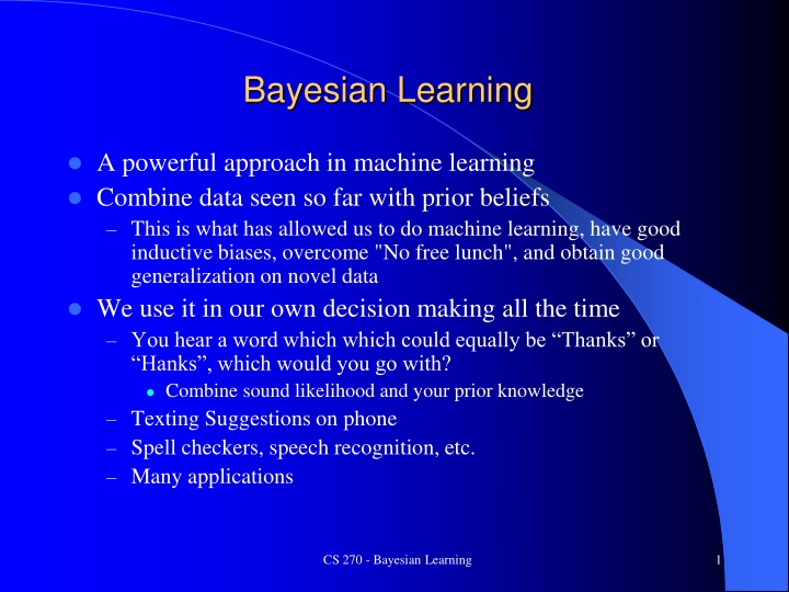
Bayesian Learning A powerful approach in machine learning Combine data seen so far with prior beliefs This is what has allowed us to do machine learning, have good inductive biases, overcome "No free lunch", and obtain good generalization on novel data We use it in our own decision making all the time You hear a word which which could equally be Thanks or Hanks , which would you go with? Combine sound likelihood and your prior knowledge Texting Suggestions on phone Spell checkers, speech recognition, etc. Many applications CS 270 - Bayesian Learning 1

Bayesian Classification P(c|x) - Posterior probability of output class c given the input vector x The discriminative learning algorithms we have learned so far try to approximate this directly P(c|x) = P(x|c)P(c)/P(x) Bayes Rule A true probability Seems like more work but often calculating the right hand side probabilities can be reasonable and advantageous P(c) - Prior probability of class c How do we know? Just count up and get the probability for the Training Set Easy! P(x|c) - Probability likelihood of data vector x given that the output class is c Later we will discuss ways to calculate this likelihood P(x) - Prior probability of the data vector x This is a normalizing term to get an actual probability. In practice we drop it because it is the same for each class c (i.e. independent), and we are mostly interested in which class c maximizes P(c|x). CS 270 - Bayesian Learning 2

Bayesian Classification Example Assume we have 100 examples in our Training Set with two output classes Good and Bad, and 80 of the examples are of class good. We want to figure out P(c|x) ~ P(x|c)P(c) Thus our priors are: CS 270 - Bayesian Learning 3

Bayesian Classification Example Assume we have 100 examples in our Training Set with two output classes Good and Bad, and 80 of the examples are of class good. Thus our priors are: P(Good) = .8 P(Bad) = .2 P(c|x) = P(x|c)P(c)/P(x) Bayes Rule Now we are given an input vector x which has the following likelihoods P(x|Good) = .3 P(x|Bad) = .4 What should our output be? CS 270 - Bayesian Learning 4

Bayesian Classification Example Assume we have 100 examples in our Training Set with two output classes Good and Bad, and 80 of the examples are of class good. Thus our priors are: P(Good) = .8 P(Bad) = .2 P(c|x) = P(x|c)P(c)/P(x) Bayes Rule Now we are given an input vector x which has the following likelihoods P(x|Good) = .3 P(x|Bad) = .4 What should our output be? Try all possible output classes and see which one maximizes the posterior using Bayes Rule: P(c|x) = P(x|c)P(c)/P(x) Drop P(x) since it is the same for both P(Good|x) = P(x|Good)P(Good) = .3 .8 = .24 P(Bad|x) = P(x|Bad)P(Bad) = .4 .2 = .08 CS 270 - Bayesian Learning 5

Bayesian Intuition Bayesian vs. Frequentist Bayesian allows us to talk about probabilities/beliefs even when there is little data, because we can use the prior What is the probability of a nuclear plant meltdown? What is the probability that BYU will win the national championship? As the amount of data increases, Bayes shifts confidence from the prior to the likelihood Requires reasonable priors in order to be helpful We use priors all the time in our decision making Unknown coin: probability of heads? (over time?) CS 270 - Bayesian Learning 6

Bayesian Learning of ML Models Assume H is the hypothesis space, h a specific hypothesis from H, and D is all the training data P(h|D) - Posterior probability of h, this is what we usually want to know in a learning algorithm (i.e. model selection) P(h|D) = P(D|h)P(h)/P(D) Bayes Rule P(h) - Prior probability of the hypothesis/model independent of D - do we usually know? Could assign equal probabilities Could assign probability based on an inductive bias (e.g. simple hypotheses have higher probability) Thus regularization is in the equation! P(D|h) - Probability likelihood of data given the hypothesis Just use the accuracy of the model h on the data D P(D) - Prior probability of the data P(h|D) increases with P(D|h) and P(h). In learning when seeking to discover the best h given a particular D, P(D) is the same and can be dropped. CS 270 - Bayesian Learning 7

Bayesian Learning Learning (finding) the best model the Bayesian way For Machine Learning the likelihood P(D|h) is usually measured using the accuracy of the hypothesis on the training data If the hypothesis is very accurate on the data, that implies that the data is more likely given that particular hypothesis Maximum a posteriori (MAP) hypothesis hMAP = argmaxh HP(h|D) = argmaxh HP(D|h)P(h)/P(D) = argmaxh HP(D|h)P(h) Maximum Likelihood (ML) Hypothesis hML = argmaxh HP(D|h) MAP = ML if all priors P(h) are equally likely (uniform priors) Note that the prior can be like an inductive bias (i.e. simpler hypotheses are more probable) For Bayesian learning, overfitting handled in the equation. Note regularization similarities. CS 270 - Bayesian Learning 8

Bayesian Learning (cont) Brute force approach is to test each h H to see which maximizes P(D|h)P(h) P(D|h)P(h) is called the Relative Posterior and is not the real probability without the normalizing P(D) Can still get the real probability (if desired) by normalization if there is a limited number of hypotheses Assume only two possible hypotheses h1 and h2 The true posterior probability of h1 would be ?(?| 1)?( 1) ?(?| 1) + ?(?| 2) ?( 1 |?) = CS 270 - Bayesian Learning 9

Example of MAP Hypothesis Assume only 3 possible hypotheses in hypothesis space H Given a data set D which h do we choose? Maximum Likelihood (ML): argmaxh HP(D|h) Maximum a posteriori (MAP): argmaxh HP(D|h)P(h) Likelihood P(D|h) Prior P(h) Relative Posterior P(D|h)P(h) H .6 .3 .18 h1 .9 .2 .18 h2 .7 .5 .35 h3 CS 270 - Bayesian Learning 10

Example of MAP Hypothesis True Posteriors Assume only 3 possible hypotheses in hypothesis space H Given a data set D Likelihood P(D|h) Prior P(h) Relative Posterior P(D|h)P(h) True Posterior P(D|h)P(h)/P(D) H .6 .3 .18 .18/(.18+.18+.35) = .18/.71 = .25 .18/.71 = .25 h1 .9 .2 .18 h2 .7 .5 .35 .35/.71 = .50 h3 CS 270 - Bayesian Learning 11

Prior Handles Overfit Prior can make it so that less likely hypotheses (those likely to overfit) are less likely to be chosen Similar to regularization Minimize F(h) = Error(h) + Complexity(h) P(h|D) = P(D|h)P(h) The challenge is Deciding on priors subjective Maximizing across H which is usually infinite approximate by searching over "best h's" in more efficient time CS 270 - Bayesian Learning 12

Minimum Description Length Information theory shows that the number of bits required to encode a message i is -log2pi Call the minimum number of bits to encode message i with respect to code C: LC(i) hMAP = argmaxh H P(h) P(D|h)= argminh H - log2P(h) - log2(D|h) = argminh HLC1(h) + LC2(D|h) LC1(h) is a representation of hypothesis LC2(D|h) is a representation of the data. Since you already have h all you need is the data instances which differ from h, which are the lists of misclassifications The h which minimizes the MDL equation will have a balance of a small representation (simple hypothesis) and a small number of errors CS 270 - Bayesian Learning 13

Bayes Optimal Classifier Best question is what is the most probable classification c C for a new instance input x, rather than what is the most probable hypothesis for a data set Let all possible hypotheses vote for the instance in question, weighted by their posterior (an ensemble approach) - better than the single best MAP hypothesis ? ???, ? ?(?| ?)?( ?) ?(?) ? ???,?,? = ? ???, ? ?( ?|?) = ? ? ? ? Bayes Optimal Classification: ?????????????= argmax ? ???, ? ?( ?|?) ?? ? ? ? = argmax ?? ? ? ???, ? ?(?| ?)?( ?) ? ? Also known as the posterior predictive CS 270 - Bayesian Learning 14

Bayes Optimal Classifier Best question is what is the most probable classification c C for a new instance input x, rather than what is the most probable hypothesis for a data set Let all possible hypotheses vote for the instance in question, weighted by their posterior (an ensemble approach) - better than the single best MAP hypothesis Also known as the posterior predictive CS 270 - Bayesian Learning 15

Example of Bayes Optimal Classification ?????????????= argmax ? ???, ??(?| ?)?( ?) ?? ? ? ? Assume same 3 hypotheses with priors and posteriors as shown for a data set D with 2 possible output classes (A and B) Assume novel input instance x where h1 and h2 output B and h3 outputs A as class 1/0 output case. Which class wins and what are the probabilities? Likelihood P(D|h) Prior P(h) Posterior P(D|h)P(h) P(A) P(B) H .6 .3 .18 0 .18 = 0 1 .18 = .18 h1 .9 .2 .18 h2 .7 .5 .35 h3 Sum CS 270 - Bayesian Learning 16

Example of Bayes Optimal Classification ?????????????= argmax ? ???, ??(?| ?)?( ?) ?? ? ? ? Assume same 3 hypotheses with priors and posteriors as shown for a data set D with 2 possible output classes (A and B) Assume novel input instance x where h1 and h2 output B and h3 outputs A as class 1/0 output case. Which class wins and what are the probabilities? Likelihood P(D|h) Prior P(h) Posterior P(D|h)P(h) P(A) P(B) H .6 .3 .18 0 .18 = 0 1 .18 = .18 h1 .9 .2 .18 0 .18 = 0 1 .18 = .18 h2 .7 .5 .35 1 .35 = .35 0 .35 = 0 h3 Sum .35 .36 CS 270 - Bayesian Learning 17

Example of Bayes Optimal Classification Assume probabilistic outputs from the hypotheses for new a instance x H P(A) P(B) .3 .7 h1 h2 h3 .4 .6 .9 .1 Likelihood P(D|h) Prior P(h) Posterior P(D|h)P(h) P(A) P(B) H .6 .3 .18 .3 .18 = .054 .7 .18 = .126 h1 .9 .2 .18 .4 .18 = .072 .6 .18 = .108 h2 .7 .5 .35 .9 .35 = .315 .1 .35 = .035 h3 Sum .441 .269 CS 270 - Bayesian Learning 18

Bayes Optimal Classifiers (Cont.) No other classification method using the same hypothesis space can outperform a Bayes optimal classifier on average, given the available data and prior probabilities over the hypotheses Large or infinite hypothesis spaces make this impractical in general Also, it is only as accurate as our knowledge of the priors (background knowledge) for the hypotheses, which we often do not know But if we do have insights, priors can really help For example, it would automatically handle overfit, with no need for a validation set, early stopping, etc. Note that using accuracy, etc. for likelihood P(D|h) is also an approximation If our priors are bad, then Bayes optimal will not be optimal for the actual problem. For example, if we just assumed uniform priors, then you might have a situation where the many lower posterior hypotheses could dominate the fewer high posterior ones. However, Bayes optimal is an important theoretical concept, and it leads to many practical algorithms which are simplifications based on the concepts of full Bayes optimality (e.g. ensembles) CS 270 - Bayesian Learning 19

Nave Bayes Revisit Bayesian Classification P(c|x) = P(x|c)P(c)/P(x) P(c) - Prior probability of class c How do we know? Just count up and get the probability for the Training Set Easy! P(x|c) - Probability likelihood of data vector x given that the output class is c We use ? ?1, ,?? ?? as short for ? ?1= ???1, ,??= ?????? How do we really do this? If x is real valued? If x is nominal we can just look at the training set and count to see the probability of x given the output class c but how often will all x s values be the same? Which will also be the problem if we bin real valued inputs CS 270 - Bayesian Learning 20

Nave Bayes Classifier ????= argmax ?? ? ? ???1, ,?? = argmax ? ?1, ,?? ???(??) ?? ? Note we are not considering h H, rather just collecting statistics from the data set Given a training set, P(cj) is easy to calculate How about P(x1, , xn|cj)? Most cases would be either 0 or 1 Key "Na ve" leap: Assume conditional independence of the attributes ? ?1, ,????= ?(??|??) ? ???= argmax ? ?? ? ???? ?? ? ? P(Thin, Red, Meat | Good) = P(Thin | Good) * P(Red | Good) * P(Meat | Good) There is usually sufficient data to get accurate values for independent terms CS 270 - Bayesian Learning 21

Nave Bayes Classifier While conditional independence is not typically a reasonable assumption (heart rate and blood pressure) Low complexity simple approach Need only store all P(cj) and P(xi|cj) terms Assume nominal features for the moment Easy to calculate the |attribute values| |classes| terms There is usually enough data to make the independent terms reasonably accurate Effective and common for many large applications (Document classification, etc.) CS 270 - Bayesian Learning 22

Nave Bayes Example For the given training set: 1. Create a table of the statistics needed to do Na ve Bayes 2. What would be the best output for a new instance which is Large and Blue? (e.g. the class which wins the argmax) 3. What is the true probability for each output class (P or N) for Large and Blue? Size (L, S) L Color (R,G,B) R Output (P,N) N S B P S G N L R N L G P ???= argmax ?(??) ?(??|??) ?? ? ? What do we need? CS 270 - Bayesian Learning 23

?(??) P(P) P(N) ?(??|??) P(Size=L|P) Size (L, S) L Color (R,G,B) R Output (P,N) N P(Size=S|P) P(Size=L|N) P(Size=S|N) S B P P(Color=R|P) S G N P(Color=G|P) L R N P(Color=B|P) L G P P(Color=R|N) P(Color=G|N) ???= argmax ?(??) ?(??|??) P(Color=B|N) ?? ? ? CS 270 - Bayesian Learning 24

**Challenge Question** Finish and give the true Probabilities of P and N for Size = L and Color = B ?(??) P(P) 2/5 P(N) 3/5 ?(??|??) P(Size=L|P) 1/2 Size (L, S) L Color (R,G,B) R Output (P,N) N P(Size=S|P) 1/2 P(Size=L|N) 2/3 P(Size=S|N) S B P P(Color=R|P) S G N P(Color=G|P) L R N P(Color=B|P) L G P P(Color=R|N) P(Color=G|N) ???= argmax ?(??) ?(??|??) P(Color=B|N) ?? ? ? P(N) = ? P(P) = 2/5 * 1/2 * P(Color = B|P) = ? CS 270 - Bayesian Learning 25

**Challenge Question** Finish and give the true Probabilities of P and N for Size = L and Color = B ?(??) P(P) 2/5 P(N) 3/5 ?(??|??) P(Size=L|P) 1/2 Size (L, S) L Color (R,G,B) R Output (P,N) N P(Size=S|P) 1/2 P(Size=L|N) 2/3 P(Size=S|N) 1/3 S B P P(Color=R|P) 0/2 S G N P(Color=G|P) 1/2 L R N P(Color=B|P) 1/2 L G P True Probabilities P(P) = .1/(.1+0) = 1 P(N) = 0/(.1+0) = 0 P(Color=R|N) 2/3 P(Color=G|N) 1/3 ???= argmax ?(??) ?(??|??) P(Color=B|N) 0/3 ?? ? ? P(N) = 3/5 * 2/3 * 0/3 = 0 P(P) = 2/5 * 1/2 * 1/2 = 1/10 CS 270 - Bayesian Learning 26

Nave Bayes Homework For the given training set: 1. Create a table of the statistics needed to do Na ve Bayes 2. What would be the best output for a new instance which is Small and Blue? (e.g. the class which wins the argmax) 3. What is the true probability for each output class (P or N) for Small and Blue? Size (L, S) L Color (R,G,B) R Output (P,N) P S B P S B N L R N L B P L G N ???= argmax ?(??) ?(??|??) S B P ?? ? ? CS 270 - Bayesian Learning 27

Nave Bayes (cont.) Can normalize to get the actual na ve Bayes probability Continuous data? - Can discretize a continuous feature into bins, thus changing it into a nominal feature and then gather statistics normally How many bins? - More bins is good, but need sufficient data to make statistically significant bins. Thus, base it on data available Could also assume data is Gaussian and compute the mean and variance for each feature given the output class, then each P(xi|cj) becomes ?(xi| xi|cj, 2xi|cj) Not good if data is multi-modal CS 270 - Bayesian Learning 28

Infrequent Data Combinations Would if there are 0 or very few cases of a particular xi=v|cj (nv/n)? (nv is the number of instances with output cj where xi = attribute value v and n is the total number of instances with output cj) Should usually allow every case at least some finite probability since it could occur in the test set, else the 0 terms will dominate the product Could replace nv/n with the Laplacian:(nv+1)/(n+|V|) Where |V| is the number of possible attribute values Thus if nv/n is 0/10 and xi has three attribute values, the Laplacian would be 1/13. CS 270 - Bayesian Learning 29

Nave Bayes (cont.) No training - Just gather the statistics from the data set and then apply the Na ve Bayes classification equation to any new instance Easier to have many attributes since not building a model (eg MLP), and the amount of statistics gathered grows linearly with the number of attribute values (# attribute values # classes) - Thus natural for applications like text classification which can be represented with huge numbers of input attributes. Though Na ve Bayes is limited by first order assumptions, it is still often used and gives reasonable results in many large real-world applications CS 270 - Bayesian Learning 30

Text Classification Example A text classification approach Want P(class|document) How to represent document? CS 270 - Bayesian Learning 31

Text Classification Example A text classification approach Want P(class|document) - Use a "Bag of Words" approach order independence assumption (valid?) Variable length input of query document is fine Calculate bag of words for every word/token in the language and each output class based on the training data. Words that occur in testing but do not occur in the training data are ignored. Good empirical results. Can drop filler words (the, and, etc.) and words found less than z times in the training set. CS 270 - Bayesian Learning 32

Text Classification Example A text classification approach Want P(class|document) - Use a "Bag of Words" approach order independence assumption (valid?) Variable length input of query document is fine Calculate bag of words for every word/token in the language and each output class based on the training data. Words that occur in testing but do not occur in the training data are ignored. Good empirical results. Can drop filler words (the, and, etc.) and words found less than z times in the training set. P(class|document) P(class|BagOfWords) //assume word order independence = P(BagOfWords|class)*P(class)/P(document) //Bayes Rule P(class)* P(word|class) // But BagOfWords usually unique // P(document) same for all classes // Thus Na ve Bayes CS 270 - Bayesian Learning 33

Text Classification Example A text classification approach Want P(class|document) - Use a "Bag of Words" approach order independence assumption (valid?) Variable length input of query document is fine Calculate bag of words for every word/token in the language and each output class based on the training data. Words that occur in testing but do not occur in the training data are ignored. Good empirical results. Can drop filler words (the, and, etc.) and words found less than z times in the training set. P(class|document) P(class|BagOfWords) //assume word order independence = P(BagOfWords|class)*P(class)/P(document) //Bayes Rule P(class)* P(word|class) // But BagOfWords usually unique // P(document) same for all classes // Thus Na ve Bayes CS 270 - Bayesian Learning 34

Less Nave Bayes NB uses just 1st order features - assumes conditional independence calculate statistics for all P(xi|cj)) |attributes| |attribute values| |output classes| nth order - P(xi, ,xn|cj) - assumes full conditional dependence |attributes|n |attribute values| |output classes| Too computationally expensive - exponential Not enough data to get reasonable statistics - most cases occur 0 or 1 time 2nd order? - compromise - P(xixk|cj) - assume only low order dependencies |attributes|2 |attribute values| |output classes| More likely to have cases where number of xixk|cj occurrences are 0 or few, could just use the higher order features which occur often in the data 3rd order, etc. How might you test if a problem is conditionally independent? Could just compare against 2nd or higher order. How far off on average is our assumption P(xixk|cj) = P(xi|cj) P(xk|cj)? CS 270 - Bayesian Learning 35

Bayesian Belief Nets Can explicitly specify where there is significant conditional dependence - intermediate ground (all dependencies would be too complex and not all are truly dependent). If you can get both of these correct (or close) then it can be a powerful representation. Important research area - CS 677 Specify causality in a DAG and give conditional probabilities from immediate parents (causal) Still can work even if causal links are not that accurate, but more difficult to get accurate conditional probabilities Belief networks represent the full joint probability function for a set of random variables in a compact space - Product of recursively derived conditional probabilities If given a subset of observable variables, then you can infer probabilities on the unobserved variables - general approach is NP-complete - approximation methods are used Gradient descent learning approaches for conditionals. Greedy approaches to find network structure. CS 270 - Bayesian Learning 36