Bayesian Model Selection in Factorial Designs: Simplifying Box and Meyer's Approach

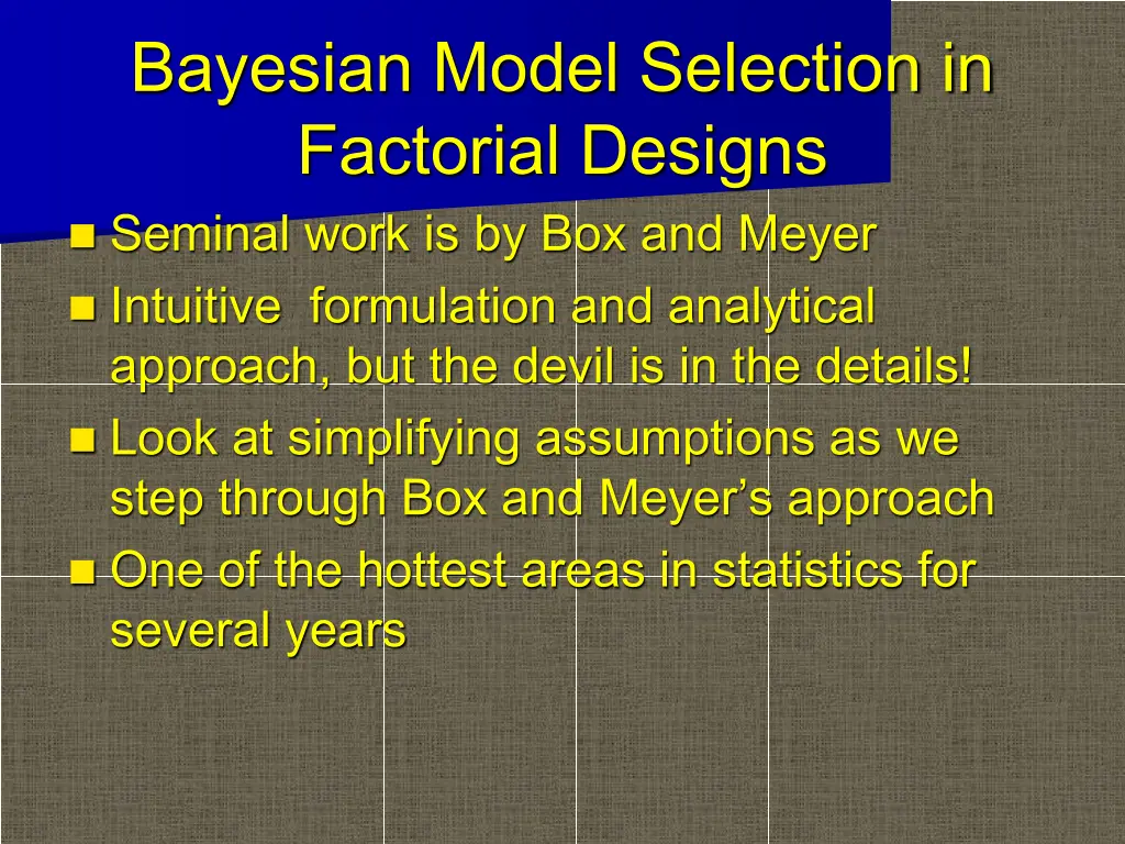
Bayesian Model Selection in Factorial Designs Seminal work is by Box and Meyer Intuitive formulation and analytical approach, but the devil is in the details! Look at simplifying assumptions as we step through Box and Meyer s approach One of the hottest areas in statistics for several years

Model Domain There are 2k-p=n possible (fractional) factorial models, denoted as a set {Ml}. To simplify later calculations, we usually assume that the only active effects are main effects, two-way effects or three-way effects This assumption is already in place for low- resolution fractional factorials

Active Effects in Models Each Mldenotes a set of active effects (both main effects and interactions) in a hierarchical model. We will use Xik=1 for the high level of effect k and Xik=-1 for the low level of effect k.

Normal Linear Model We will assume that the response variables follow a linear model with normal errors given model M:Yi~N(X Xi , ) Xiand are model-specific, but we will use a saturated model in what follows.

Likelihood Function The likelihood for the data given the parameters has the following form 2n 1 1 ( ) 2 2s2Yi- L(b,s,Y)= - Xib 2ps2exp 1 2s2Y -Xb i=1 1 ) Y -Xb ( ( ) = n2exp - ( ) 2ps2

Bayesian Paradigm Unlike in classical inference, we assume the parameters, , are random variables that have a prior distribution, f ( ), rather than being fixed unknown constants. In classical inference, we estimate by maximizing the likelihood L( |y)

Posterior Density Estimation using the Bayesian approach relies on updating our prior distribution for after collecting our data y. The posterior density, by an application of Bayes rule, is proportional to the product of the familiar data density and the prior density: ( ) fX|Q(x |q)fQ(q) fQ|Yq |y

Bayes Estimator The Bayes estimate of minimizes Bayes risk the expected value (with respect to the prior) of loss function L( ). Under squared error loss, the Bayes estimate is the mean of the posterior distribution: q y ( ) = EQ|YQ

Prior Likelihood The Bayesian prior for models is quite straightforward. The prior probability that r effects are active in the model, given each is active with prior probability is r p ( ) ( ) n-1-r=C11-p n-1 L(p)=C1pr1-p 1-p

Prior Likelihood for Linear Model Parameters Since we re using a Bayesian approach, we need priors for and as well b0~ N 0,s2e ( bj~ N 0,g2s2 ( s ~ g s ( ), g s ( ) s-a ), e =10-6 )

Zellners g-prior For non-orthogonal designs, it s common to use Zellner s g-prior for : ( ) ( ) -1 bj~ N 0,g2s2X'X Note that we did not assign priors to or

Complete Data Likelihood We can combine f( , , ) and f(Y| , , ) to obtain the full likelihood L( , , ,Y) 2n-1+a 2 n-1 r1 1 2s2Q(b) p 1 L(b,s,M,Y)=C 1-p g 2ps2 exp -

Expansion of Complete Data Likelihood Terms

Posterior Model Derivation Our goal is to derive the posterior distribution of M given Y, which first requires integrating out and . Rn L(M |Y) L(M,Y)= L(b,s,M,Y)dbds = 0 ( ) -1 2 XX +G n-1 r1 p C ( ) (n-1+a) 2 1-p g ( ) -1 XX +G Q XY

Posterior Model Partition The first term is a penalty for model complexity (smaller is better) The second term is a measure of model fit (smaller is better)

Posterior Model Distribution and are still present. We will fix ; the method is robust to the choice of is selected to minimize the probability of no active factors

Posterior Model Selection With L(M|Y) in hand, we can actually evaluate the P(Mi|Y) for all Mifor any prior choice of , provided the number of Miis not burdensome This is in part why we assume eligible Mi only include lower order effects.

Selection Criteria Greedy search or MCMC algorithms are used to select models when they cannot be itemized Selection criteria include Bayes Factor, Schwarz criterion, Bayesian Information Criterion Refer to R package BMA and bic.glm for fitting more general models.

Marginal Selection For each effect, we sum the probabilities for all Mithat contain that effect and obtain a marginal posterior probability for that effect. These marginal probabilities are relatively robust to the choice of .

Case Study Violin data* (24factorial design with n=11 replications) Response: Decibels Factors A: Pressure (Low/High) B: Placement (Near/Far) C: Angle (Low/High) D: Speed (Low/High) *Carla Padgett, STAT 706 taught by Don Edwards

Case Study Summary Fractional Factorial Design: A, B, and D significant AB marginal Bayesian Model Selection: A, B, D, AB, AD, BD significant All others negligible *Carla Padgett, STAT 706 taught by Don Edwards