Block Diagram Transformation Theorems and Examples

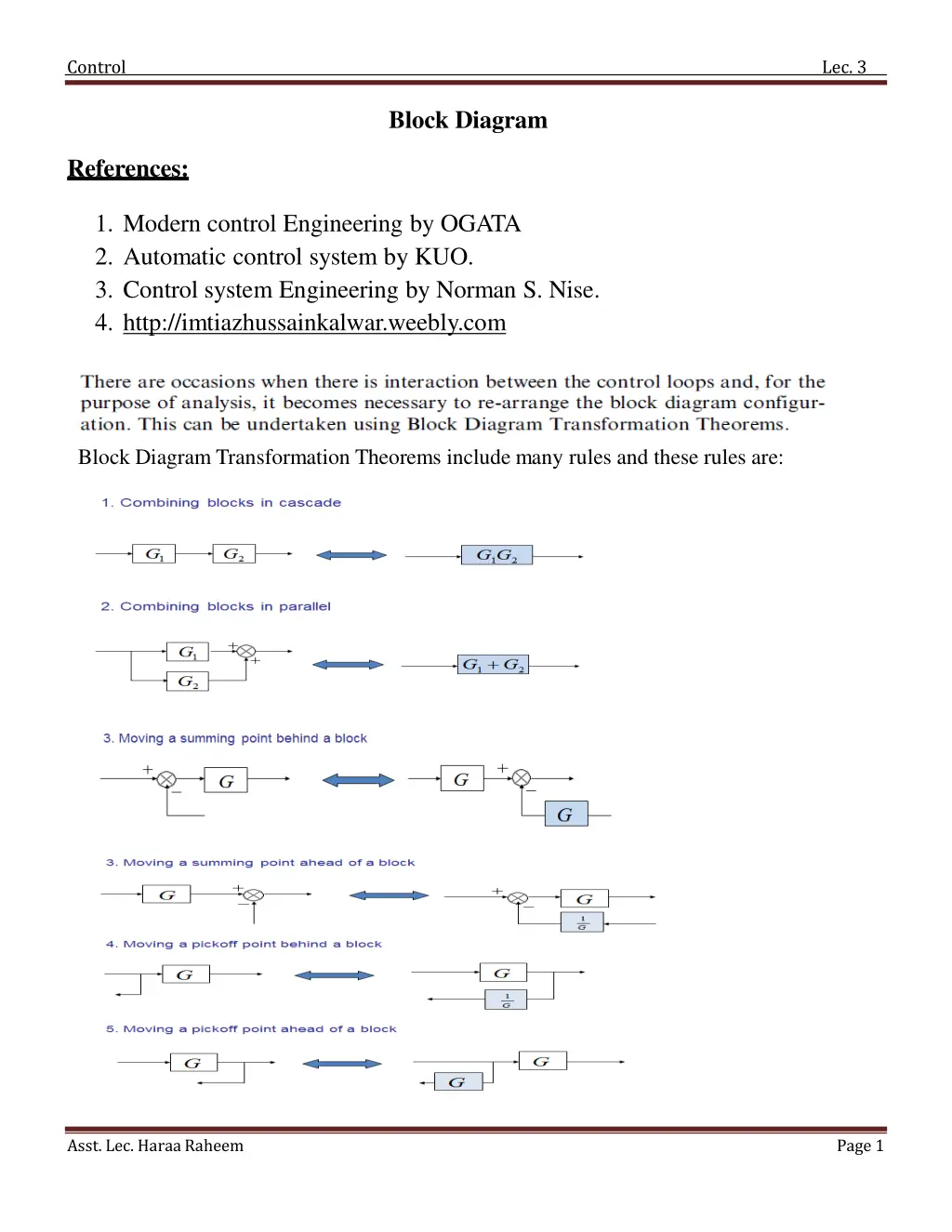
Control Lec. 3 Block Diagram References: 1. Modern control Engineering by OGATA 2. Automatic control system by KUO. 3. Control system Engineering by Norman S. Nise. 4. http://imtiazhussainkalwar.weebly.com Block Diagram Transformation Theorems include many rules and these rules are: Asst. Lec. Haraa Raheem Page 1

Control Lec. 3 Table (3.1) Block Diagram transformation theorems Asst. Lec. Haraa Raheem Page 2

Control Lec. 3 Ex1: Find the transfer function of the following block diagrams C R + G1 G2 C R G1G2 - + H1 + H2 H1+H2 R C Ex2: Find the transfer function of the following block diagrams Asst. Lec. Haraa Raheem Page 3

Control Lec. 3 R C Ex3: For the system represented by the following block diagram determine: 1. Open loop transfer function 2. Feed Forward Transfer function 3. control ratio 4. feedback ratio 5. error ratio 6. closed loop transfer function 7. characteristic equation Sol: First we will reduce the given block diagram Asst. Lec. Haraa Raheem Page 4

Control Lec. 3 K s+1 K G s+1 = 1+K s s+1 1+GH B(s) = G(s)H(s) E(s) 1. Open loop transfer function C(s)= G(s) E(s) 2. Feed Forward Transfer function = C(s ) R(s ) G(s) 3.control ratio 1+G(s)H (s) B(s) G(s)H(s) = 4. feedback ratio ( ) R(s) 1+G(s)H(s) ( ) = E(s ) R(s ) 1 5. error ratio 1+G(s)H (s) Asst. Lec. Haraa Raheem Page 5

Control Lec. 3 = C(s ) R(s ) G(s) 6. closed loop transfer function 1+G(s)H (s) 1+G(s)H(s) = 0 7. characteristic equation Ex4: Find the transfer function of the following block diagrams Asst. Lec. Haraa Raheem Page 6

Control Lec. 3 Ex5: Reduce the Block Diagram Asst. Lec. Haraa Raheem Page 7

Control Lec. 3 H.W1: Find the transfer function of the following block diagrams H.W2: Simplify the block diagram then obtain the close-loop transfer function C(S)/R(S). Multiple Input System EX1: Determine the output C due to inputs R and U using the Superposition Method sol: according to the principles of superposition, then, we must try to find the o/p considering one i/p at time Asst. Lec. Haraa Raheem Page 8

Control Lec. 3 Asst. Lec. Haraa Raheem Page 9

Control Lec. 3 Multi-Input Multi-Output System Ex1: Determine C1 and C2 due to R1 and R2. Asst. Lec. Haraa Raheem Page 10

Control Lec. 3 When R1 = 0 When R2 = 0 Asst. Lec. Haraa Raheem Page 11

Control Lec. 3 Signal Flow Graphs The block diagram is useful for graphically representing control system dynamics and is used extensively in the analysis and design of control systems. An alternate approach for graphically representing control system dynamics is the signal flow graph approach, due to S. J.Mason. It is noted that the signal flow graph approach and the block diagram approach yield the same information and one is in no sense superior to the other. Definitions: Before we discuss signal flow graphs, we must define certain terms: Node: Anode is a point representing a variable or signal. Transmittance: The transmittance is a real gain or complex gain between two nodes. Such gains can be expressed in terms of the transfer function between two nodes. Branch: Abranch is a directed line segment joining two nodes. The gain of a branch is a transmittance. Input node or source: An input node or source is a node that has only outgoing branches. Output node or sink: An output node or sink is a node that has only incoming branches. Mixed node: A mixed node is a node that has both incoming and outgoing branches. Path:Apath is a traversal of connected branches in the direction of the branch arrows. Loop: Aloop is a closed path. Loop gain:The loop gain is the product of the branch transmittances of a loop. Non touching loops: Loops are nontouching if they do not possess any common nodes. Forward path: A forward path is a path from an input node (source) to an output node (sink) that does not cross any nodes more than once. Forward path gain:A forward path gain is the product of the branch transmittances of a forward path. Figure (3.1) Signal flow graph Asst. Lec. Haraa Raheem Page 12

Control Lec. 3 Signal Flow GraphAlgebra A signal flow graph of a linear system can be drawn using the foregoing definitions. In doing so, we usually bring the input nodes (sources) to the left and the output nodes (sinks) to the right. The independent and dependent variables of the equations become the input nodes (sources) and output nodes (sinks), respectively. The branch transmittances can be obtained from the coefficients of the equations. To determine the input-output relationship, we may use Mason's formula, which will be given later, or we may reduce the signal flow graph to a graph containing only input and output nodes. To accomplish this, we use the following rules: 1. The value of a node with one incoming branch, as shown in Figure 3-1(a), is x2 = ax1. 2. The total transmittance of cascaded branches is equal to the product of all the branch transmittances. Cascaded branches can thus be combined into a single branch by multiplying the transmittances, as shown in Figure 3-1(b). 3. Parallel branches may be combined by adding the transmittances, as shown in Figure 3-1(c). 4. A mixed node may be eliminated, as shown in Figure 3-1(d). 5. Aloop may be eliminated, as shown in Figure 3-1(e). Note that x3 = bx2, x2 = ax1 + cx3 Figure 3-2 Signal flow graphs and simplifications Asst. Lec. Haraa Raheem Page 13

Control Lec. 3 x3 = abx1+bcx3 x3= (1) (2) Hence Equation (1) corresponds to a diagram having a self-loop of transmittance bc. Elimination of the self-loop yields Equation (2), which clearly shows that the overall transmittance is ab/(l - bc). Signal Flow Graphs of Control Systems: Some signal flow graphs of simple control systems are shown in Figure 3-2. For such simple graphs, the closed-loop transfer function C(s)/R(s)[ or c(s)/N(s)]can be obtained easily by inspection. For more complicated signal flow graphs, Mason's gain formula is quite useful. Figure 3-3 Block diagrams and corresponding signal flow graphs Asst. Lec. Haraa Raheem Page 14

Control Lec. 3 Mason's Gain Formula for Signal Flow Graphs The block diagram reduction technique requires successive application of fundamental relationships in order to arrive at the system transfer function. On the other hand, Mason s rule for reducing a signal-flow graph to a single transfer function requires the application of one formula. The formula was derived by S. J. Mason when he related the signal-flow graph to the simultaneous equations that can be written from the graph. The transfer function, C(s)/R(s), of a system represented by a signal-flow graph is: n i = 1 Pi i C ( s ) R ( s ) = Where n = number of forward paths. Pi = the ith forward-path gain. = Determinant of the system or is a series of summation of the untouched loops i = Determinant of the ith forward path is called the signal flow graph determinant or characteristic function = 1- (sum of all individual loop gains) + (sum of the products of the gains of all possible two loops that do not touch each other) (sum of the products of the gains of all possible three loops that do not touch each other) + and so forth with sums of higher number of non-touching loop gains i = value of for the part of the block diagram that does not touch the i-th forward path ( i = 1 if there are no non-touching loops to the i-th path.) Solution steps by Mason's rule 1. Calculate forward path gain Pi for each forward path i. 2. Calculate all loop transfer functions 3. Consider non-touching loops 2 at a time 4. Consider non-touching loops 3 at a time 5. Etc Asst. Lec. Haraa Raheem Page 15

Control Lec. 3 6. Calculate from steps 2,3,4 and 5 7. Calculate ias portion of not touching forward path i Example1: Apply Mason s Rule to calculate the transfer function of the system represented by following Signal Flow Graph C R P1 1 + P2 2 Therefore = There are three feedback loops L1 = G1G4H1, , L2 = G1G2G4H2 L3 = 2 G1G3G4H There are no non-touching loops, therefore = 1- (sum of all individual loop gains) = 1 (L1+ L2 + L3) = 1 (G1G4H1 G1G2G4H2 G1G3G4H2) Eliminate forward path-1 1 = 1- (sum of all individual loop gains)+... 1 = 1 Eliminate forward path-2 2 = 1- (sum of all individual loop gains)+... 2 = 1 Asst. Lec. Haraa Raheem Page 16

Control Lec. 3 Example-2: Determine the transfer function C/R for the block diagram below by signal flow graph techniques. Sol: The signal flow graph of the above block diagram is shown below. There are two forward paths. The path gains are The three feedback loop gains are L1= -G2H1, L2= G1G2H1, L3= -G2G3H2 No loops are non-touching, hence =1 (L1 + L2 + L3) Because the loops touch the nodes of P1, hence Since no loops touch the nodes of P2, therefore Hence the control ratio T = C/R is: Asst. Lec. Haraa Raheem Page 17

Control Lec. 3 Example-3: Find the control ratio C/R for the system given below. Sol: The signal flow graph is shown in the figure. The two forward path gains are The five feedback loop gains are L1= G1G2H1, L2= G2G3H2, L3= -G1G2G3, L4= G4H2, L5=-G1G4 There are no non-touching loops, hence =1 (L1 + L2 + L3 + L4 + L5) = 1- G1G2H1- G2G3H2+ G1G2G3- G4H2+ G1G4 All feedback loops touches the two forward paths, hence Hence the control ratio : Asst. Lec. Haraa Raheem Page 18

Control Lec. 3 H.W 1: Find the control ratio C/R for the system given below by signal flow graph techniques. H.W 2: Find the control ratio C/R for the system given below by signal flow graph techniques. Asst. Lec. Haraa Raheem Page 19

Control Lec. 3 Example 4: Apply Mason s Rule to calculate the transfer function of the system represented by following Signal Flow Graph Sol: 1.Calculate forward path gains for each forward path. P1 =G1G2G3G4 (path1) and P2 =G5G6G7G8 (path2) 2. Calculate all loop gains. L1 =G2H2, L2 =H3G3, L3 =G6H6, L4 =G7H7 3. Consider two non-touching loops. L1L3 L1L4 L2L4 L2L3 Consider three non-touching loops. 4. None. 5. Calculate from steps 2,3,4. = 1 (L1 + L2 + L3 + L4)+(L1L3 + L1L4 + L2L3 + L2L4) = 1 (G2H (G2H H 7 ) + 2 + 3G3 + G6H 6 + G2H 6 + G7H 7 + H 6 + 2G6H 2G7H H 3G3G6H H 3G3G7 7 ) 1 = 1 (L3 + 1 = 1 (G6H6 + G7H7) L4) 2 = 1 (L1 + L2) 2 =1 (G2H2 +G3H3) Asst. Lec. Haraa Raheem Page 20

Control Lec. 3 P1 1 + Y ( s ) R ( s ) P2 = 2 G1G2G3G4 1 ( G6H6 +G7H7) +G5G6G7G8 1 ( G2H2 +G3H3) 1 ( G2H2 +H3G3+G6H6 +G7H7 )+( G2H2G6H6 +G2H2G7H7 +H3G3G6H6 +H3G3G7H7) Y(s)= R(s) Example 5: Apply Mason s Rule to calculate the transfer function of the system represented by following Signal Flow Graph Sol: P1 = A32A43A54A65A76 P2 = A72 P3 = A42A54A65A76 two non-touching loops: Three non-touching loops: Asst. Lec. Haraa Raheem Page 21