BRACED Interim Monitoring & Evaluation Guidance - Webinar Summary

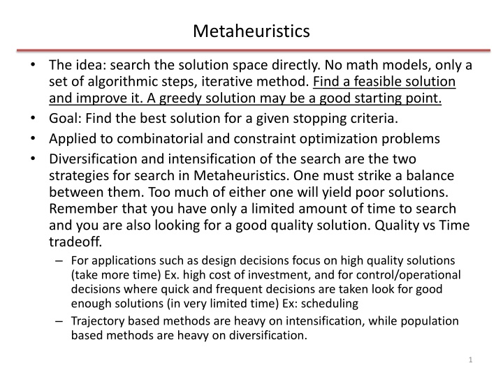
Metaheuristics The idea: search the solution space directly. No math models, only a set of algorithmic steps, iterative method. Find a feasible solution and improve it. A greedy solution may be a good starting point. Goal: Find the best solution for a given stopping criteria. Applied to combinatorial and constraint optimization problems Diversification and intensification of the search are the two strategies for search in Metaheuristics. One must strike a balance between them. Too much of either one will yield poor solutions. Remember that you have only a limited amount of time to search and you are also looking for a good quality solution. Quality vs Time tradeoff. For applications such as design decisions focus on high quality solutions (take more time) Ex. high cost of investment, and for control/operational decisions where quick and frequent decisions are taken look for good enough solutions (in very limited time) Ex: scheduling Trajectory based methods are heavy on intensification, while population based methods are heavy on diversification. 1

Setting up a heuristic search 2

Representation of a Solution and its Neighborhood Representation of solutions Vector of Binary values 0/1 Knapsack, 0/1 IP problems Vector of discrete values- Location , and assignment problems Vector of continuous values on a real line continuous, parameter optimization Permutation sequencing, scheduling, TSP Neighborhood: k-distance for vector representations For discrete values distance d(s,s )< for continuous values: sphere of radius d around s For binary vector of size n, 1-distance neighborhood of s will have n neighbors (flip one bit at a time) Ex: hypercube, neighbors of 000 are 100, 010, 001. Neighborhood: For permutation based representations k-exchange (swapping) or k-opt operator (for TSP) Ex: 2-opt: for permutations of size n, the size of the neighborhood is n(n-1)/2. The neighbors of 231 are 321, 213 and 132 for scheduling problems Insertion operator 12345 14235 Exchange operator 12345 14325 Inversion operator 123456 154326 3

Understanding complexity - Distance and Landscape For binary and flip move operators For a problem of size n, the search space size is 2n and the maximum distance of the search space is n (the maximum distance is by flipping all n values). For permutation and exchange move operators For a problem of size n, the search space size is n! and the maximum distance between 2 permutations is n-1 Landscapes Flat, plain; basin, valley; rugged, plain; rugged, valley 4

Initial solution, constraints check, and objective function Random or greedy or hybrid In most cases starting with greedy will reduce computational time and yield better solutions, but not always Sometimes random solutions may be infeasible Sometimes expertise is used to generate initial solutions Hybrid: For population-based metaheuristics a combination of greedy and random solutions is a good strategy. Constraints - feasibility check Complete vs incremental evaluation of the obj. function TSP- in every solution add all the distances to find the total distance TSP - in every solution evaluate only the change and add with previously stored sub-strings to find the total distance Straightforward or subjective, may be expensive, approximate (expected value). 5

Pick a Method The idea: search the solution space directly. No math models, only a set of algorithmic steps, iterative method. Trajectory based methods (single solution based methods) search process is characterized by a trajectory in the search space It can be viewed as an evolution of a solution in (discrete) time of a dynamical system Tabu Search, Simulated Annealing, Iterated Local search, variable neighborhood search, guided local search Population based methods Every step of the search process has a population a set of- solutions It can be viewed as an evolution of a set of solutions in (discrete) time of a dynamical system Genetic algorithms, swarm intelligence - ant colony optimization, bee colony optimization, scatter search Hybrid methods Parallel metaheuristics: parallel and distributed computing- independent and cooperative search You will learn these techniques through several examples 6

Infeasibility, Bail-out strategies, Stopping Criteria Dealing with infeasible neighborhoods Bail-out strategies from local optima Decide the stopping criteria, Stop After a fixed number of moves After a fixed number of moves show no improvements over the current best solution. When computational time runs out If you are satisfied with the current best solution 7

S-Metaheuristics single solution based Idea: Improve a single solution These are viewed as walks through neighborhoods in the search space (solution space) The walks are performed via iterative procedures that move from the current solution to the next one Iterative procedure consist of generation and replacement from a single current solution. Generation phase: A set of candidate solutions C(s) are generated from the current solution s by local transformation. Replacement phase: Selection of s is performed from C(s) such that the obj function f(s ) is better than f(s). s C(s) s The iterative process continues until a stopping criteria is reached The generation and replacement phases may be memoryless. Otherwise some history of the search is stored for further generation of candidate solutions. Key elements: define the solution representation, neighborhood structure, and the initial solution. 8

Local search Hill climbing (descent), iterative improvement Select an initial solution Selection of the neighbor that improves the solution (and its obj func) Best improvement (steepest ascent/descent). Exhaustive exploration of the neighborhood (all possible moves). Pick the best one with the largest improvement. First improvement (partial exploration of the neighborhood) Random selection evaluate a few randomly selected neighbors and select the best among them. Great method if there are not too many local optimas. Issues: search time depends on initial solution and not good if there are many local optimas. 9

Local search Maximize f(x)= x3-60x2+900x 0<x 40 Use binary search Starting solution 10001 = 24+ 20 = f (17) = 2774 Find the neighbors for 10001 Solution : local optima is 10000 = f(16) = 3136 But global optima is 01010 = f(10)= 4000 11111 = f(31), what about 32 .40. The solution does not permit all possible values of x to be evaluated. 111111 = f(63), 41 ..63 are infeasible as per constraint rejection startegy. 10

Local search for IP Solve Max Z = 3x1 +2x2+4x3+5x4+6x5 s.t. 2x1 +3x3 300 2x1 + 4x4 +8x5 250 4x2+5x3-3x4 150 0 xi 100, xi are integers 1015solutions 1010 possible solutions with some infeasible ones -LP relaxation (linear objective function and linear constraints) -Solution representation for IP is {x1, ..,x5}. Branch and bound, cutting plane . Branch and bound only if a lower and upper bound can be found it becomes an exhaustive search -Metaheuristic solution representation 7 digit-Binary representation for each variable. x1 = 1111111 = f(x1) = with 101 and above infeasible. Similarly for other variables. otherwise 127 (max), If the objective function and constraints are nonlinear ? Lower and upper bounds are difficult to evaluate. Metaheuristics will still work. 11

Escaping local optimas Accept nonimproving neighbors Tabu search and simulated annealing Iterating with different initial solutions Multistart local search, greedy randomized adaptive search procedure (GRASP), iterative local search Changing the neighborhood Variable neighborhood search Changing the objective function or the input to the problem in a effort to solve the original problem more effectively. Guided local search 12

Tabu search Decide solution representation Initialize a solution Decide a neighborhood generation method and generate neighbors Decide Tabu list = list the forbidden swaps from a fixed number of previous moves (usually between 5 and 9 swaps for large problems), too few will result in cycling and too many may be unduly constrained. Decide Tabu tenure of a move= number of iterations for which a move is forbidden. Decide the stopping criteria Stopping criterion: Stop after a fixed number of moves or after a fixed number of moves show no improvements over the current best solution. 13

TSP NY 0 13 16 8 Miami 13 0 14 15 Dallas 16 14 0 9 Chicago 8 15 9 0 New York Miami Dallas Chicago initial solution 1342 obj fnc 53 Distance in hundreds of miles 14

Knapsack - Tabu search and SA Knapsack item 1 2 3 wt 4 3 5 benefit 11 7 12 max wt 10 lb maximize benefit initial solution 1 1 0 benefit =18 15

Tabu search Single Machine Scheduling problems Single machine, n jobs, minimize total weighted tardiness, a job when started must be completed, N-P hard problem, n! solutions Completion time Cj Due date dj Processing time pj Weight wj Release date rj Tardiness Tj = max (Cj-dj, 0) Total weighted tardiness = wj . Tj The value of the best schedule is also called aspiration criterion 16

Tabu Search Single machine scheduling example Single machine, 4 jobs, minimize total weighted tardiness, a job when started must be completed, N-P hard problem, 4! Solutions Use adjacent pair-wise flip operator Tabu list last two moves cannot be swapped again. Jobs j 1 2 3 pj 10 10 13 dj 4 2 1 wj 14 12 1 4 4 12 12 Initial solution 2143 weighted tardiness = 500 17

Parallel machines m machines and n jobs Machines are in parallel, identical and can process all types of jobs Ex. 2 machines, 4 jobs Jobs j pj dj 1 9 2 9 3 12 4 3 10 8 5 28 wj 14 12 1 12 Initial solution 3142 Weighted tardiness 163 =7*1+13*12= 163 3 2 12 21 1 4 12 9 18

Flow shop m machines and n jobs Machines are along a conveyor belt, may not be identical and can process all types of jobs. Ex. 2 machines, 4 jobs, processing times equal on both machines (not necessary though). No buffer or bypass allowed Each job must flow first on machine 1 then on machine 2 Jobs j pj dj 1 9 2 9 3 12 4 3 10 8 5 28 wj 14 12 1 12 Initial solution 3142 3 1 4 2 Weighted tardiness 881 =19*1+23*14+8*12+37*12 12 21 24 33 3 1 4 2 12 24 33 36 45 19

Set-covering problems Applications Airline crew scheduling: Allocate crews to flight segments Political districting Airline scheduling Truck routing Location of warehouses Location of a fire station Set covering example using Tabu search 20

Tabu search with variants Static and dynamic size of tabu list Short term memory stores recent history of solutions to prevent cycling. Not very popular because of high data storage requirements. Medium term memory Intensification of search around the best found solutions. Only as effectives as the landscape structure. Ex: intensification around a basin is useless. Long term memory Encourages diversification. Keeps an account of the frequency of solutions (often from the start of the search) and encourages search around the most frequent ones. 21