Canadian Regional Climate Model Overview
The Canadian Regional Climate Model (CRCM) is a mesoscale meteorological model that solves fully elastic Eulerian equations using a semi-Lagrangian semi-implicit scheme. First developed in the 1990s, it allows for longer time steps, improved efficiency, and is driven by simulations from the Canadian Centre for Climate modeling and analysis. This model uses a terrain-following scaled height vertical coordinate system with a grid box length of 45 km and a polar stereographic projection. The governing equations of the model include velocity components of wind, Coriolis parameter, specific pseudokinetic energy, heat, moisture sources/sinks, momentum sources/sinks, gravity, gas constant for dry air, temperature, specific humidity, and more. The model also implements Gal-Chen terrain-following coordinate and Eulerian equations for momentum, continuity, thermodynamic, and moisture.
Download Presentation

Please find below an Image/Link to download the presentation.
The content on the website is provided AS IS for your information and personal use only. It may not be sold, licensed, or shared on other websites without obtaining consent from the author.If you encounter any issues during the download, it is possible that the publisher has removed the file from their server.
You are allowed to download the files provided on this website for personal or commercial use, subject to the condition that they are used lawfully. All files are the property of their respective owners.
The content on the website is provided AS IS for your information and personal use only. It may not be sold, licensed, or shared on other websites without obtaining consent from the author.
E N D
Presentation Transcript
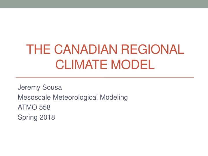
THE CANADIAN REGIONAL CLIMATE MODEL Jeremy Sousa Mesoscale Meteorological Modeling ATMO 558 Spring 2018
Introduction to the CRCM First runs took place in the 1990s Fully compressible and non-hydrostatic Solves fully elastic Eulerian equations using a semi- Lagrangian semi-implicit scheme Allows the use of longer time steps than traditional Eulerian schemes improved efficiency Simulations from the Canadian Centre for Climate modeling and analysis (CCCma) second-generation GCM (GCMII) are used to drive the CRCM The same physical parameterization package as the CCCma GCMII is used
Introduction to the CRCM (Cont.) Uses a terrain-following scaled height vertical coordinate system (Gal-Chen and Somerville 1975) Grid box length: 45 km Uses polar stereographic projection
Model Governing Equations U,V,w: velocity components of wind q=ln(p/p0) f: Coriolis parameter K=(U2+V2)/2 specific pseudokinetic energy L,E: heat & moisture sources/sinks Fx,Fy,Fz: momentum sources/sinks g: gravity R: gas constant for dry air =R/cp where cp is specific heat at constant pressure T: temperature M: specific humidity Momentum Thermodynamic Continuity Moisture
Mapping Terms S=m2: projection metric term m=(1+sin 0)/(1+sin ) where m is a map scale factor Total derivative is given by: Components are defined as: Model wind components are defined as:
Terrain-Following Gal-Chen Coordinate Used to implement terrain into CRCM Defined by the following equation: Z is scaled height coordinate, h0 is topographic height, and H is top of model atmosphere Apply chain rule and substitute into Euler equations to obtain
Gal-Chen Eulerian Equations Momentum Continuity Thermodynamic Moisture
Term Expansion Start by decomposing fields into basic and perturbation states (q=q*+q ; T=T*+T ) Substitute expanded fields into Euler equations, apply Reynold s averaging Adding linear terms accounting for elastic and gravity waves yields
Expanded Euler Equations Momentum Moisture Continuity Coordinate Adjustment Thermodynamic
Semi-Implicit Semi-Lagrangian Scheme Idea: Express LHS of governing equations as averages of fields on grid points at current forecast time and upstream values at past times. Derivatives computed by: , , and are Lagrangian displacements are calculated by iteratively solving the following equations:
SISL Equations Momentum Moisture Continuity Coordinate Correction Thermodynamic
Temporal Discretizations Equations are computed and grouped into terms Q (time t+ t), P (time t- t), and R (time t) Equations at forecast time (Q) are computed by the following relation:
Q Governing Equations Momentum adjustment factor for uncentered averaging Continuity Thermodynamic Moisture Coordinate Adjustment
P Governing Equations Momentum Continuity Thermodynamic Moisture Coordinate Adjustment
R Governing Equations Momentum Continuity Thermodynamic Moisture Coordinate Adjustment
Computed Variables where
Parameterizations Fx, Fy, Fz are friction terms and represent subgrid-scale processes that impact momentum equations Momentum fluxes computed using an eddy diffusivity free atmosphere formulation with a surface drag coefficient formulation Unresolved gravity waves are parameterized by adding drag force to the flow L term represents diabatic heating, latent heat flux, and turbulent/convective vertical heat flux Three infrared bands and one visible band Land surface parameterizatoins: CLASS 2.7 (Verseghy 1991)
References Caya, D., and R. Laprise, 1999: A Semi-Implicit Semi- Lagrangian Regional Climate Model: The Canadian RCM. Mon. Wea. Rev., 127, 341-362. Gal-Chen, T. et R. C. Somerville, 1975: On the Use of a Coordinate Transformation for the Solution of Navier- Stockes. J. Comput. Phys., 17, 209-228.
