Capital Allocation to Risky Assets in Investments: Overview and Decision-Making
Explore the process of capital allocation in risky assets, including top-down approach, asset allocation decisions, and security selection. Understand risk aversion, portfolio construction, passive strategies, and the role of the capital market line. Delve into risk and risk aversion, utility values, and the assessment of available risky portfolios.

Download Presentation

Please find below an Image/Link to download the presentation.
The content on the website is provided AS IS for your information and personal use only. It may not be sold, licensed, or shared on other websites without obtaining consent from the author. If you encounter any issues during the download, it is possible that the publisher has removed the file from their server.
You are allowed to download the files provided on this website for personal or commercial use, subject to the condition that they are used lawfully. All files are the property of their respective owners.
The content on the website is provided AS IS for your information and personal use only. It may not be sold, licensed, or shared on other websites without obtaining consent from the author.
E N D
Presentation Transcript
Chapter Six Capital Allocation to Risky Assets INVESTMENTS | BODIE, KANE, MARCUS INVESTMENTS | BODIE, KANE, MARCUS
Three Steps in Investment Decisions Top-down Approach Capital Allocation Decision Allocate funds between risky and risk-free assets Made at higher organization levels I. II. Asset Allocation Decision Distribute risky investments across asset classes small-cap stocks, large-cap stocks, bonds, & foreign assets III. Security Selection Decision Select particular securities within each asset class Made at lower organization levels INVESTMENTS | BODIE, KANE, MARCUS INVESTMENTS | BODIE, KANE, MARCUS 6-2
Chapter Overview Risk aversion and its estimation Two-step process of portfolio construction Composition of risky portfolio Capital allocation between risky and risk-free assets Passive strategies and the capital market line (CML) INVESTMENTS | BODIE, KANE, MARCUS INVESTMENTS | BODIE, KANE, MARCUS 6-3
Risk and Risk Aversion Speculation Taking considerable risk for a commensurate gain Parties have heterogeneous expectations Gamble Bet on an uncertain outcome for enjoyment Parties assign the same probabilities to the possible outcomes INVESTMENTS | BODIE, KANE, MARCUS 6-4
Risk and Risk Aversion Utility Values Investors are willing to consider: Risk-free assets Speculative positions with positive risk premiums Portfolio attractiveness increases with expected return and decreases with risk What happens when return increases with risk? INVESTMENTS | BODIE, KANE, MARCUS INVESTMENTS | BODIE, KANE, MARCUS 6-6
Example INVESTMENTS | BODIE, KANE, MARCUS INVESTMENTS | BODIE, KANE, MARCUS 6-7
Table 6.1 Available Risky Portfolios Each portfolio receives a utility score to assess the investor s risk/return trade off INVESTMENTS | BODIE, KANE, MARCUS INVESTMENTS | BODIE, KANE, MARCUS 6-8
Risk Aversion and Utility Values Utility Function U = Utility E(r) = Expected return on the asset or portfolio A = Coefficient of risk aversion 2= Variance of returns = A scaling factor ( ) 12 = A 2 U E r INVESTMENTS| BODIE, KANE, MARCUS INVESTMENTS| BODIE, KANE, MARCUS 6-9
Investor Types Risk Averse Investors: 0 A Risk-Neutral Investors: 0 A = Risk Lovers: A 0 Where A = Coefficient of risk aversion INVESTMENTS| BODIE, KANE, MARCUS INVESTMENTS| BODIE, KANE, MARCUS 6-10 6-10
Table 6.2 Utility Scores of Portfolios with Varying Degrees of Risk Aversion INVESTMENTS| BODIE, KANE, MARCUS INVESTMENTS| BODIE, KANE, MARCUS 6-11
Estimating Risk Aversion Use questionnaires PDF Observe individuals decisions when confronted with risk Observe how much people are willing to pay to avoid risk INVESTMENTS| BODIE, KANE, MARCUS INVESTMENTS| BODIE, KANE, MARCUS 6-12
Capital Allocation Across Risky and Risk-Free Portfolios Asset Allocation The choice among broad asset classes that represents a very important part of portfolio construction The simplest way to control risk is to manipulate the fraction of the portfolio invested in risk-free assets versus the portion invested in the risky assets INVESTMENTS| BODIE, KANE, MARCUS INVESTMENTS| BODIE, KANE, MARCUS 6-13
Basic Asset Allocation Example Total market value Risk-free money market fund $300,000 $90,000 Equities Bonds (long-term) Total risk assets $113,400 $96,600 $210,000 113 $ , 400 96 $ 600 , = = = = . 0 54 W . 0 46 W E B 210 $ 000 , 210 $ 00 , INVESTMENTS| BODIE, KANE, MARCUS INVESTMENTS| BODIE, KANE, MARCUS 6-14
Basic Asset Allocation Example Let y = Weight of the risky portfolio, P, in the complete portfolio (1-y) = Weight of risk-free assets 210 $ 000 , $ 90 000 , = = y = = 7 . 0 1 3 . 0 y 300 $ 000 , 300 $ 000 , 113 $ , 400 $ 96 600 , = : 378 . E = : 322 . B 300 $ 000 , 300 $ 000 , INVESTMENTS| BODIE, KANE, MARCUS INVESTMENTS| BODIE, KANE, MARCUS 6-15
The Risk-Free Asset Only the government can issue default-free securities A security is risk-free in real terms only if its price is indexed and maturity is equal to investor s holding period T-bills viewed as the risk-free asset Money market funds also considered risk-free in practice INVESTMENTS| BODIE, KANE, MARCUS INVESTMENTS| BODIE, KANE, MARCUS 6-16
Portfolios of One Risky Asset and a Risk-Free Asset It s possible to create a complete portfolio by splitting investment funds between safe and risky assets Let y = Portion allocated to the risky portfolio, P (1 - y) = Portion to be invested in risk-free asset, F INVESTMENTS| BODIE, KANE, MARCUS INVESTMENTS| BODIE, KANE, MARCUS 6-17
Example rf = 7% rf = 0% p = 22% E(rp) = 15% y = % in p (1-y) = % in rf INVESTMENTS| BODIE, KANE, MARCUS
Expected Returns for Combinations = + ( ) c E r ( ) (1 p yE r ) y r f rc = complete or combined portfolio For example, y = .75 E(rc) = .75(.15) + .25(.07) = .13 or 13% INVESTMENTS| BODIE, KANE, MARCUS
Standard Deviation of Complete Portfolio c= y p INVESTMENTS| BODIE, KANE, MARCUS
Combinations Without Leverage Combinations Without Leverage If y = .75, then c = .75(.22) = .165 or 16.5% If y = 1 c = 1(.22) = .22 or 22% If y = 0 c = (.22) = .00 or 0% INVESTMENTS| BODIE, KANE, MARCUS
Capital Allocation Line (CAL) E(rc) = yE(rp) + (1 y)rf = rf +[(E(rp) rf)]y (1) c= y p y = c/ p (2) From (1) and (2) E(rc) = rf +[(E(rp) - rf)/ p] c (CAL) INVESTMENTS| BODIE, KANE, MARCUS INVESTMENTS| BODIE, KANE, MARCUS 6-22
One Risky Asset and a Risk-Free Asset: Example E(rc) = rf +[(E(rp) - rf)/ p] c = 7 + [(15 7)/22] c = 7 + (8/22) c ( ) P E r r 8 22 f = = Slope P INVESTMENTS| BODIE, KANE, MARCUS INVESTMENTS| BODIE, KANE, MARCUS 6-23
Figure 6.3 The Investment Opportunity Set INVESTMENTS| BODIE, KANE, MARCUS INVESTMENTS| BODIE, KANE, MARCUS 6-24
Capital Allocation Line with Leverage Borrow at the Risk-Free Rate and invest in stock. Using 50% Leverage, rc= (-.5) (.07) + (1.5) (.15) = .19 c= (1.5) (.22) = .33 INVESTMENTS| BODIE, KANE, MARCUS
The Opportunity Set with Differential Borrowing and Lending Rates Capital allocation line with leverage Lend at rf= 7% and borrow at rf= 9% Lending range slope = 8/22 = 0.36 Borrowing range slope = 6/22 = 0.27 CAL kinks at P INVESTMENTS| BODIE, KANE, MARCUS INVESTMENTS| BODIE, KANE, MARCUS 6-26
Figure 6.4 The Opportunity Set with Differential Borrowing and Lending Rates INVESTMENTS| BODIE, KANE, MARCUS INVESTMENTS| BODIE, KANE, MARCUS 6-27
Risk Tolerance and Asset Allocation The investor must choose one optimal portfolio, C, from the set of feasible choices Expected return of the complete portfolio: ( ) f c r r E + = ( ) p r y E r f Variance: = y 2 c 2 2 p INVESTMENTS| BODIE, KANE, MARCUS INVESTMENTS| BODIE, KANE, MARCUS 6-28
Table 6.4 Utility Levels for Various Positions in Risky Assets INVESTMENTS| BODIE, KANE, MARCUS INVESTMENTS| BODIE, KANE, MARCUS 6-29
Figure 6.5 Utility as a Function of Allocation to the Risky Asset, y INVESTMENTS| BODIE, KANE, MARCUS INVESTMENTS| BODIE, KANE, MARCUS 6-30
Analytical Solution U = E(rc) (1/2)A c2 (1) where E(rc) = yE(rp) + (1-y)rf c = y p (2) (3) Substituting (2) and(3) into (1), we obtain U = yE(rp) + (1-y)rf (1/2)A(y p)2 From dU/dy = E(rp) rf Ay p2 = 0, y* = (E(rp) rf)/A p2 INVESTMENTS| BODIE, KANE, MARCUS INVESTMENTS| BODIE, KANE, MARCUS 6-31
y* = (E(rp) rf)/Ap2 = (0.15 0.07)/4(0.22)2 = 0.41 E(rc) = y*E(rp) + (1-y*)rf = 0.41(0.15) + (1-0.41)(0.07) = 0.1028 c = y* p = 0.41(0.22) = 0.0902 Hence, U = E(rc) (1/2)A c2 = 0.1028 (1/2)4(0.0902)2 = 0.08653 INVESTMENTS| BODIE, KANE, MARCUS INVESTMENTS| BODIE, KANE, MARCUS 6-32
Indifference curve We can trace combinations of E(rc) and c for given values of U and A. From U = E(rc) (1/2)A c2 E(rc) = U + (1/2)A c2 Example: E(rc) = 0.05 + (1/2)(2) c2 INVESTMENTS| BODIE, KANE, MARCUS INVESTMENTS| BODIE, KANE, MARCUS 6-33
Table 6.5 Spreadsheet Calculations of Indifference Curves INVESTMENTS| BODIE, KANE, MARCUS INVESTMENTS| BODIE, KANE, MARCUS 6-34
Figure 6.6 Indifference Curves for U = .05 and U = .09 with A = 2 and A = 4 INVESTMENTS| BODIE, KANE, MARCUS INVESTMENTS| BODIE, KANE, MARCUS 6-35
Figure 6.7 Finding the Optimal Complete Portfolio (A = 4) INVESTMENTS| BODIE, KANE, MARCUS INVESTMENTS| BODIE, KANE, MARCUS 6-36
Table 6.6 Expected Returns on Four Indifference Curves and the CAL INVESTMENTS| BODIE, KANE, MARCUS INVESTMENTS| BODIE, KANE, MARCUS 6-37
Passive Strategies: The Capital Market Line E(rc) = rf +[(E(rM) - rf)/ M] c The passive strategy avoids any direct or indirect security analysis Supply and demand forces may make such a strategy a reasonable choice for many investors A natural candidate for a passively held risky asset would be a well-diversified portfolio of common stocks such as the S&P 500 INVESTMENTS| BODIE, KANE, MARCUS INVESTMENTS| BODIE, KANE, MARCUS 6-38
Passive Strategies: The Capital Market Line The Capital Market Line (CML) Is a capital allocation line formed investment in two passive portfolios: 1. Virtually risk-free short-term T-bills (or a money market fund) 2. Fund of common stocks that mimics a broad market index INVESTMENTS| BODIE, KANE, MARCUS INVESTMENTS| BODIE, KANE, MARCUS 6-39
Passive Strategies: The Capital Market Line From 1926 to 2018, the passive risky portfolio offered an average risk premium of 8.34% with a standard deviation of 20.36%, resulting in a reward-to-volatility ratio of .41 Index Funds https://www.fool.com/investing/how-to- invest/index-funds/average-return/ INVESTMENTS| BODIE, KANE, MARCUS INVESTMENTS| BODIE, KANE, MARCUS 6-40


")


 – rf)/Aσp2")