Categorical Data Analysis and Goodness-of-Fit Testing Methods
Explore the world of categorical data analysis with Xuhua Xia from the University of Ottawa. Learn about various statistical approaches such as exact tests, chi-square tests, and gamma distributions. Discover relationships within data sets and understand the significance of chi-square distributions. Enhance your knowledge of statistical testing methods for analyzing data effectively.
Download Presentation

Please find below an Image/Link to download the presentation.
The content on the website is provided AS IS for your information and personal use only. It may not be sold, licensed, or shared on other websites without obtaining consent from the author. If you encounter any issues during the download, it is possible that the publisher has removed the file from their server.
You are allowed to download the files provided on this website for personal or commercial use, subject to the condition that they are used lawfully. All files are the property of their respective owners.
The content on the website is provided AS IS for your information and personal use only. It may not be sold, licensed, or shared on other websites without obtaining consent from the author.
E N D
Presentation Transcript
Categorical data analysis Xuhua Xia University of Ottawa http://dambe.bio.uottawa.ca
Goodness-of-Fit test A sample of fish from a large lake Male: 15 Female 5 H0: 1:1 sex ratio Three approaches: 1. Exact test 2. X2-test (chi-square test) 3. G2-test (likelihood ratio chi-square test) Common in all significance tests (except for exact test that considers all possible events): 1. a statistic measuring the deviation of observation from expectation based on H0 2. a distribution for the statistic so that a p value can be obtained.
Exact test (All scenarios) Male Female Binomial 9.53674E-07 1.90735E-05 0.000181198 0.001087189 0.004620552 0.014785767 0.036964417 0.073928833 0.120134354 0.160179138 0.176197052 0.160179138 0.120134354 0.073928833 0.036964417 0.014785767 0.004620552 0.001087189 0.000181198 1.90735E-05 9.53674E-07 Male: 15 Female 5 H0: 1:1 sex ratio 0 1 2 3 4 5 6 7 8 9 20 19 18 17 16 15 14 13 12 11 10 0.020695 10 11 12 13 14 15 16 17 18 19 20 9 8 7 6 5 4 3 2 1 0 0.020695 Xuhua Xia
Gamma distribution 1.2 f(x|0.5,2) 2 distribution with 1 degree of freedom f(x|1,2) f(x|1,10) Exponential distribution with = 1/10 f(x|5,2) 2 distribution with 10 degrees of freedom Exponential distribution with = 1/2 1 0.8 f(x) 0.6 ? ?|?,? =?? 1? ? ? ; ?,? > 0;0 ? ?? ? 0.4 ?? 1? ??? ? = 0.2 0 mean = , var = 2 0 0 5 10 15 20 25 30 35 40 x ? 2 1? ? 2 ? 2 ? ?|? =? 2,? = 2 =? Two special cases: 1. With = /2 and = 2 2 distribution 2. With =1 exponential distribution ,> 0;? 0 ? 2 2 ? ?|? = 1,? =? ? ? ; ? > 0;0 ? ?
Chi-square Distribution 2 distribution is a special case of gamma distribution with = /2 and = 2. It has a mean of and variance 2 . 0.6 = 2 0.5 0.4 = 4 f(x) 1 / x 0.3 x e = 8 ( ; , ) p x = ( ) 0.2 0.1 /2 1 /2 x x e ( ; /2,2) p x = 0 /2 ( /2) 2 0 5 10 15 20 x x = 1 ( ; /2,2) p x v p dx The p value in chi-square test: 0 In EXCEL, p = CHISQ.DIST.RT (x,DF) = 1-GAMMA.DIST (x,DF/2,2,true) In R: 1-pchisq(x,df)
Relationships If we sample n values from a standard normal distribution to get z1, z2, ..., zn, the statistic Szz below follows 2 distribution with n degrees of freedom (DF): ???= ?1 Naturally, if n = 1, then Szz would be 2-distributed with 1 degree of freedom. 2+ ?2 2+ + ?? 2 This implies that, if we sample n values from a normal distribution with mean and variance 2, then Sxx follows 2 distribution with n degrees of freedom: ?? ?2 ?2 ?2 ? 1 ?2 ?2 gives us SS. This relationship is useful for attaching confidence interval for 2 ? ?? ?2 ?? ?2 ?2 ?? ?2 ?2 = ?=1 ???= + + s2 is the sample variance. Multiplying it by (n-1) ???=
Confidence interval for 2 ? 1 ?2 ?2 2 ???= ~?? 1 ? 1 ?2 ?2 ? 1 ?2 ?? 1,? 2 2 1 ? = ? ?? 1,? ? 1 ?2 ?? 1,1 ? ?? 1,1 ? 2 2 ?2 = ? 2 2 2 2 UL LL For example, if n = 80, s2 = 20, then to attach 95% CI, n<-80; s2<-20; X2<-qchisq(c(0.025, 0.975),n-1) CI<-rev((n-1)*s2/X2); CI.sd<-sqrt(CI) This is the general approach to attach confidence interval for a parameter with no known distribiton by finding a statistic with a known distribution,
X2 statistic ? ?2 ? 15 102 10 5 102 10 breaks count expCount 1 73698 68268.95 2 14714 16001.13 3 4 7372 3776.425 5 3029 2015.295 6 7 8 938 347.3237 9 10 218 113.4394 11 12 13 26 22.05145 14 15 16 17 ?2= = + = 5 ? ?? ?2 ?2 0 7403.469 ???= ?=1 80000 70000 0 1104.144 0 615.4907 "it is necessary to regard each cell value as normally distributed with a variance equal to the expected value" 60000 50000 40000 0 197.7939 30000 0 65.42834 0 37.91134 20000 10000 Yates (1934) 0 0 12.86803 0 7.529946 0 4.416869 5 2.596267 0 2 4 6 8 10 12 14 16 18 count expCount DF <- 1; N<-100000 rbin<-rbinom(N,20,0.5) X2<-2*(rbin-10)^2/10 # A sample of 20 with n hits and (20-n) misses res<-hist(X2); numClass<-length(res$counts) breakPoints<-res$breaks[2:(numClass+1)] qtile<-pchisq(breakPoints,DF) expCount<-qtile*N for(i in numClass:2) expCount[i]<-expCount[i]-expCount[i-1] md<-data.frame(breaks=breakPoints,count=res$counts,expCount=expCount) write.table(md,"clipboard",sep="\t")
N=10, p = 0.5, Nexp = 10 x 0 1 2 3 4 5 6 7 8 9 p'. P. P(X2)/2 0.000783 0.005706 0.02889 0.102952 0.263545 Diff1 P(X2')/2 0.002213 0.013428 0.056923 0.171391 0.375915 Diff2 0.000977 0.009766 0.043945 0.117188 0.205078 0.246094 0.205078 0.117188 0.043945 0.009766 0.000977 0.000977 0.010742 0.054688 0.171875 0.376953 0.623047 0.828125 0.945313 0.989258 0.999023 -0.000194 -0.005036 -0.025798 -0.068923 -0.113408 0.001237 0.002686 0.002236 -0.000484 -0.001038 1 10 1 Recalculated from Table I in Yates 1934 Xuhua Xia
N=20, p = 0.25, Nexp: 5, 15 x1 x2 20 0.003171 0.003171 6.666667 0.004912 0.001740 19 0.021141 0.021141 4.266667 0.019434 -0.001708 3.266667 0.035351 0.014209 18 0.066948 0.066948 2.4 0.060668 -0.006280 1.666667 0.098353 0.031405 17 0.133896 0.225156 1.066667 0.150850 -0.074306 16 0.189685 0.414842 0.266667 0.302788 -0.112053 0.066667 0.398127 -0.016715 15 0.202331 14 0.168609 0.382827 0.266667 0.302788 -0.080039 0.066667 0.398127 0.015299 13 0.112406 0.214218 1.066667 0.150850 -0.063368 12 0.060887 0.101812 2.4 0.060668 -0.041144 1.666667 0.098353 -0.003459 11 0.027061 0.040925 4.266667 0.019434 -0.021492 3.266667 0.035351 -0.005575 10 0.009922 0.013864 6.666667 0.004912 -0.008953 9 0.003007 0.003942 9.6 0.000973 -0.002969 8.066667 0.002254 -0.001688 8 0.000752 0.000935 13.06667 0.000150 -0.000785 11.26667 0.000395 -0.000541 7 0.000154 0.000184 17.06667 0.000018 -0.000166 6 0.000026 0.000030 21.6 0.000002 -2.8E-05 19.26667 5.68E-06 -2.4E-05 5 3.426E-06 3.81E-06 26.66667 1.21E-07 -3.7E-06 24.06667 4.65E-07 -3.3E-06 4 3.569E-07 3.87E-07 32.26667 6.72E-09 -3.8E-07 3 2.799E-08 2.96E-08 38.4 2.88E-10 -2.9E-08 35.26667 1.44E-09 -2.8E-08 2 1.555E-09 1.61E-09 45.06667 9.52E-12 -1.6E-09 41.66667 5.41E-11 -1.6E-09 1 5.457E-11 5.55E-11 52.26667 2.42E-13 -5.5E-11 0 9.095E-13 9.09E-13 60 4.74E-15 p'. P. P(X2)/2 Diff1 X2' 5.4 0.010068 0.006897 P(X2')/2 Diff2 X2 0 1 2 3 4 5 6 7 8 9 0.6 0.219289 -0.005867 0.6 0.219289 0.005071 10 11 12 13 14 15 16 17 18 19 20 5.4 0.010068 -0.003796 15 5.38E-05 -0.000130 29.4 2.94E-08 -3.6E-07 48.6 1.57E-12 -5.4E-11 3.5E-14 -8.7E-13 -9E-13 56.06667 "From the nature of these discrepancies it is clear that no simple modification of the correction for continuity will materially improve the approximations obtained." -Yates (1934)
G2 statistic Male: 15 Female 5 H0: 1:1 sex ratio 20! 15!5!0.5150.55 20! 15!5!0.75150.255 ?2= ?1= Male Female 0 1 2 3 4 5 6 7 8 9 10 11 12 13 14 15 16 17 18 19 20 Binomial 20 9.53674E-07 19 1.90735E-05 18 0.000181198 17 0.001087189 16 0.004620552 15 0.014785767 0.020695 14 0.036964417 13 0.073928833 12 0.120134354 11 0.160179138 10 0.176197052 9 0.160179138 8 0.120134354 7 0.073928833 6 0.036964417 5 0.014785767 0.020695 4 0.004620552 3 0.001087189 2 0.000181198 1 1.90735E-05 0 9.53674E-07 20! 15!5! + 15ln 0.75 + 5ln 0.25 = 1.59785 ???1= ?? 20! 15!5! + 15ln 0.5 + 5ln 0.5 = 4.21409 ???2= ?? ?? ?? ?2= 2 ???1 ???2 = 5.232481=2 ???? ? = 0.022169 2 15 102 10 5 102 10 ?? ?? ?? ?2= = + = 5 ? = 0.025347 p values from G2 and X2 tests are too small
Williams' q: n=10, p = 0.5 ? = 1 +?2 1 m: number of classes; n: sample size; : DF 6?? male female p'. P. P(G2)/2 Diff1 P(G2')/2 0.00014 Diff2 G2 0 1 2 3 4 5 6 7 8 9 10 0.000977 0.000977 13.86294 9.83188E-05 9 0.009766 0.010742 7.361284 0.003332159 8 0.043945 0.054688 3.854895 0.024800514 7 0.117188 0.171875 1.645658 0.099775495 6 0.205078 0.376953 5 0.246094 0.623047 4 0.205078 0.828125 3 0.117188 0.945313 1.645658 2 0.043945 0.989258 3.854895 1 0.009766 0.999023 7.361284 0 0.000977 1 13.86294 -0.000878 -0.007410 0.004051 -0.029887 0.027678 -0.072100 -0.114107 0.267859 -0.000837 -0.006691 -0.027009 -0.066575 -0.109094 0.1053 0.40271 0.262846435 0 0.40271 1 10 The correction is consistently in the right direction, but not quite sufficient the p values are still consistently smaller than they should be.
Williams' q: n=20, p = 0.25 p'. P. P(G2)/2 0.000347 -0.002825 0.008179 -0.012962 0.044333 -0.022614 0.137605 -0.087551 0.298323 -0.116519 Diff.1 G2' P(G2') Diff.2 G2 male female 0 1 2 3 4 5 6 7 8 9 20 19 18 17 16 15 14 13 12 11 10 0.003171 0.003171 0.021141 0.021141 0.066948 0.066948 0.133896 0.225156 0.189685 0.414842 0.202331 0.168609 0.382827 0.112406 0.214218 0.060887 0.101812 0.027061 0.040925 0.009922 0.013864 0.003007 0.003942 0.000752 0.000935 0.000154 0.000184 0.000026 0.000030 5 3.426E-06 4 3.569E-07 3 2.799E-08 2 1.555E-09 1 5.457E-11 0 9.095E-13 11.50728 5.763898 2.898413 1.190593 0.280084 11.22662 5.623315 2.82772 1.161554 0.273253 0.000403 -0.002768 0.008862 -0.012280 0.046325 -0.020623 0.140572 -0.084584 0.300579 -0.114263 0.256058 0.989989 2.164613 3.756752 5.753641 8.151201 10.95351 14.17334 17.83385 21.97225 26.64678 31.95174 38.05401 45.31394 55.45177 0.306421 -0.076407 0.159872 -0.054346 0.070610 -0.031202 0.026297 -0.014628 0.008227 -0.005637 0.002152 -0.001791 0.000467 -0.000468 0.000083 -0.000100 0.000012 1.38E-06 1.22E-07 7.9E-09 3.44E-10 8.39E-12 4.79E-14 0.249813 0.965843 2.111817 3.665123 5.613309 7.952391 10.68635 13.82765 17.39888 21.43634 25.99686 31.17243 37.12586 44.20872 54.09929 0.308603 -0.074224 0.16286 -0.051359 0.073083 -0.028729 0.027781 -0.013144 0.008912 -0.004952 0.002401 -0.001541 0.00054 -0.000396 0.0001 -0.000084 1.52E-05 1.83E-06 1.71E-07 1.18E-08 5.54E-10 1.48E-11 9.53E-14 10 11 12 13 14 15 16 17 18 19 20 9 8 7 6 -1.7E-05 -2.4E-06 -2.6E-07 -2.2E-08 -1.3E-09 -4.7E-11 -8.6E-13 -1.4E-05 -2E-06 -2.2E-07 -1.8E-08 -1.1E-09 -4.1E-11 -8.1E-13 3.81E-06 3.87E-07 2.96E-08 1.61E-09 5.55E-11 9.09E-13 Xuhua Xia
Tea-tasting & Fisher's exact test Characters: Dr. Muriel Bristol (21/Apr/1888 15/Mar/1950), Ronald Fisher (17/Feb/1890 29/Jul1962), William Roach who married Bristol in 1923. Location: Rothamsted Experimental Station Time: 1919 (The year Fisher moved to the station, two years after his marriage to Ruth Eileen) Act 1: Fisher, Bristol and Roach were in line to get tea. Fisher got his tea from a tea urn and offered it to Bristol who declined saying that she preferred tea with milk added to the cup before tea. Fisher did not think that adding milk before or after would make any difference, but Bristol insisted that it did and she could tell the difference. Roach proposed to test her. Act 2: An experimental protocol was set up haphazardly, ending with Roach declaring that Bristol's claim was confirmed. The two married soon. Act 3: Fisher thought long and hard, and proposed a protocol to do the test vigorously, leading to Fisher's exact test. Act 4: A group of students trying to understand what it is......
Fisher's experimental setup Expt setup Tea 1st Milk 1st a c 4 Bristol's pickTea 1st b d 4 4 4 8 Milk 1st Identify the four cups with tea poured first, leading to materialized a and b values which could be a b 4 0 3 1 2 2 1 3 0 4 outcomes? Question: What are the probabilities associated with each of these five possible Xuhua Xia
1. Brute-Force binomial approach Experimental outcome: a = 4, b = 0: Probability of 1st correct pick: p1 = 4/8 Probability of 2nd correct pick: p2 = 3/7 Probability of 3rd correct pick: p3 = 2/6 Probability of 4th correct pick: p4 = 1/5 p(a=4,b=0) = p1*p2*p3*p4 = 0.014286. Claim considered confirmed. Experimetnal outcome: a = 3, b = 1: Scenario1 W C C C p Scenario2 C W C C p Scenario3 C C W C p Scenario4 C C C W p 4/8 4/7 3/6 2/5 4/8 4/7 3/6 2/5 4/8 3/7 4/6 2/5 4/8 3/7 2/6 4/5 The probability of each scenario is obtained by multiplying the p values: 0.057143. The probability for all 4 scenarios is 0.057143*4 = 0.228571. The probability of Bristol doing this good and better is p = 0.014286 + 0.228571= 0.242857: Claim not supported (but not rejected). One-tailed test: no need to consider the other extreme
2. Combinatorics approach a = 4, b = 0: There are 8 way has all four cups being chosen correctly. p = 1/70 = 0.014286. Claim considered confirmed. = 70 ways of choosing 4 cups out of 8. Only one 4 a = 3, b = 1: There are 4 first cups, and 4 milk-first cups, i.e., 16 combinations. p = 16/70 = 0.228571. The probability of Bristol doing this good and better is p = 0.014286 + 0.228571= 0.242857. Claim not supported (but not rejected). =4 ways of choosing 3 cups out of the four tea- 3 =4 ways of choosing 1 cup out of the four 1 One-tailed test
3. Use hypergeometric distribution Binomial distribution: (p + q)n: p does not change with sampling. Hypergeometric distribution: when population size is small and sampling is done without replacement, then p changes with sampling as we have seen with #1 (binomial approach). Three parameters: N: population size (= 8 in our tea-tasting example) K: number of "white balls" (or successes) in the population (=4 in the tea-tasting example n: sample size (=4 in our tea-tasting example) The probability of obtain k succeses is then: 4 4 8 4 4 4 8 4 8 4 4 3 8 4 ? ? ? ? ? ? ? ? 1 ? 4 4,4,8 = = 70= 0.014286 ? ? ?,?,? = 4 3 =16 70= 0.228571 ? 3 4,4,8 = Xuhua Xia
Fisher's exact test Expt setup Tea 1st Milk 1st a c a+c C1 R1, R2, C1, C2: marginal totals. Tea 1st Milk 1st b d a+b c+d R1 R2 Bristol's pick b+d C2 n ? + ? ? c + d ? ? + ? ? c + d ? ? + ? ! ? + ? ! ? + ? ! ? + ? ! ?!?!?!?!?! ? = = = ? ? ? + ? ? + ? 4 0 4 0 4 4 4 4 8 ? =4!4!4!4! 4!4!8! = 0.014286 4!4!4!4! 3!1!1!3!8!= 0.228571 3 1 4 1 3 4 4 4 8 ? =
Contingency Table Treat Success Yes 273 289 138 No 77 61 562 A B 350 350 700 The null hypothesis: Success is independent of Treatment (i.e., the success rate is the same for both treatment). The null hypothesis can be tested with the Chi-square test of goodness-of-fit. Expected frequencies (the test should be done on counts, not on proportions). Degree of freedom X2 value: 0 if the data is perfectly consistent with the null hypothesis. p: the probability of obtaining the observed X2 value and more extreme ones given that the null hypothesis is true, i.e., ?(? ?2|?0). Xuhua Xia
X2-test of a Contingency Table? Treat Success Yes 273 289 562 For 2-test, Eij should be equal or greater than 5. No 77 61 138 A B 350 350 700 R C n 350 138 700 R C n i j = = = = , . ., e g E 69 E 1 2 12 ij Do hand-calculation of X2. 2 ( ) n E = ij ij What is the df associated with the test? 2 E ij df = (r-1)(c-1) Xuhua Xia
Formulas for different statistics 2 ( ) 11 22 n n n n n n n n n = for 2 2 table 2 12 21 1 2 O 1 2 2 ( ) E N N c r ij ij = 2 E = = 1 1 i j ij 2 n | | n 11 22 n n 11 21 n n 2 = for 2 2 table 2 c n n n n Statistic for significance tests 1 2 1 2 ( ) 2 | 0.5 | O E E ij ij = 2 c ij O E N N C R ij = 2 2 ln G O ij = = 1 1 i j ij N N N N c c r r = + 2 ln( ) ln( ) ln( ) ln( ) n n R R C C n n ij ij i i i i = = = = 1 1 1 1 i j n n i j 11 22 n n n n n n = 2 2 ; 12 21 for tables Indices of association as effect size: Phi coefficient Contingency coefficient Cramer's V 1 2 1 2 2 = C + 2 n 2 = V min( 1, 1) n r c
R functions md<-read.table("http://dambe.bio.uottawa.ca/teach/bio8102_download/KidneyStoneLumped.txt",header=T) Treat Success Freq 1 A Yes 273 2 A No 77 3 B Yes 289 4 B No 61 tab1<-xtabs(Freq~.,md) Success Treat No Yes A 77 273 B 61 289 chisq.test(tab1,correct=T) Pearson's Chi-squared test with Yates' continuity correction '.' ==All other variables in the data frame, equivalent in this case to xtabs(Freq~Treat+Success) data: tab1 X-squared = 2.0308, df = 1, p-value = 0.1541 library(MASS) #log-linear models are needed for > 2-D tables loglm(~Treat+Success,tab1) # Get likelihood ratio chi-square, i.e., G2 if(!require(vcd)) {install.packages("vcd"); library(vcd) } assocstats(tab1) # get Phi, C, and V Phi-Coefficient : 0.057 Contingency Coeff.: 0.057 Cramer's V : 0.057
Fisher's exact test for 2-D table Another way of forming contingency table 1st: row 2nd: column Kidney<-matrix(c(77, 61, 273, 289), nrow = 2,dimnames = list(Treat = c("A", "B"),Success = c("No", "Yes"))) Kidney # To check data input Treat No Yes A 77 273 B 61 289 fisher.test(Kidney, alternative = "greater") fisher.test(Kidney, alternative = "less") fisher.test(Kidney, alternative = "two.sided") data: Kidney p-value = 0.154 alternative hypothesis: true odds ratio is not equal to 1 95 percent confidence interval: 0.9036408 1.9806450 sample estimates: odds ratio 1.335713 fisher.test(Kidney, conf.level = 0.95)$conf.int [1] 0.9036408 1.9806450 attr(,"conf.level") [1] 0.95 No<-77+61;Yes<-273+289; n<-61+289; p<-0 for(i in 0:61) p=p+dhyper(i,No,Yes,n) for(i in 61:n) ...
Assignment: Sex and Hair Color GENDER | Black | Blond | Brown | Red | Total ---------+--------+--------+--------+--------+ Female | 55 | 64 | 65 | 16 | 200 ---------+--------+--------+--------+--------+ Male | 32 | 16 | 43 | 9 | 100 ---------+--------+--------+--------+--------+ Total 87 80 108 25 300 COLOR Assignment: Arrange the data and save to a text file, read in to R, format into an R table use xtabs, and use Pearson chi-square (with Yates' continuity correction) and likelihood ratio chi-square to test the null hypothesis of independence. Compute Phi, contingency coefficient and Cramer's V (Print the slide, fill in the values and conclude) Chi-square: DF: p: Likelihood ratio chi-square: DF: p: Phi: C: V:
Why are there more blonde females? An evolutionary explanation A genetic explanation A simple chemical explanation The limitation of statistics Xuhua Xia
Log-linear model Preferred statistical tool for analyzing multi-way contingency table Use likelihood ratio test to choose the best model Main effects and interactions can be interpreted in a similar manner as ANOVA R functions: loglin (available in base package) loglm (available in MASS package) Xuhua Xia
3-D Table # C. R. Charig et al. 1986. Br Med J (Clin Res Ed) 292: 879 882 # http://dambe.bio.uottawa.ca/teach/bio8102_download/KidneyStone.txt # Treatment A: all open procedures # Treatment B: percutaneous nephrolithotomy # Question: which treatment is better? Treat Success StoneSize Freq A Yes Small A No Small B Yes Small B No Small A Yes Large A No Large B Yes Large B No Large 81 6 234 36 192 71 55 25 Xuhua Xia
3-D Table (log-linear model) md<-read.table("http://dambe.bio.uottawa.ca/teach/bio8102_download/KidneyStone.txt",header=T) tab1<-xtabs(Freq~.,md) full model with list(c(1,2,3)) would fits the data perfectly. # loglin compares each model against full model fit<-loglin(tab1,list(c(1,2),c(1,3),c(2,3))) 1-pchisq(fit$lrt,fit$df) # if p> : fine without 3-way interaction. 0.3153416 fit<-loglin(tab1,list(c(1,3),c(2,3))) # reduced model 1-pchisq(fit$lrt,fit$df) # if p> : fine without 1*2? 0.1781455 fit<-loglin(tab1,list(c(1,2),c(2,3))) # reduced model 1-pchisq(fit$lrt,fit$df) # if p> : fine without 1*3? 0 fit<-loglin(tab1,list(c(1,2),c(1,3))) # reduced model 1-pchisq(fit$lrt,fit$df) # if p> : fine without 2*3? 2.041195e-07 > tab1 , , StoneSize = Large Success Treat No Yes A 71 192 B 25 55 , , StoneSize = Small Success Treat No Yes A 6 81 B 36 234 library(MASS) # full model is Treat*StoneSize*Success fit<-loglm(~Treat*StoneSize+Success*StoneSize,tab1)
2-factor associations (1,2) association: Treatment:Success 93% vs 87% and 73% vs 69%: small difference Small Large AOS 81 6 87 93% PN 234 36 270 87% AOS 192 71 263 73% PN 55 25 80 69% Success Yes No Total %Success (2,3) association: Success:StoneSize (93% vs 73% and 87% vs 69%: substantial difference Success Yes No AOS 81 192 273 30% PN 234 55 289 81% AOS 6 71 77 8% PN 36 25 61 59% Small Large Total %Small (1,3) association: StoneSize:Treatment 30% vs 81% and 8% vs 59%: substantial difference Xuhua Xia
Cochran-Armitage-trend-test # Assess the effect of a carcinogenic drug on inducing lung cancer in mice: # Dose (0,1,2), LungCancer(no=0, yes=1) library("coin") lungtumor <- data.frame(dose = rep(c(0, 1, 2), c(40, 50, 48)), tumor = c(rep(c(0, 1), c(38, 2)), rep(c(0, 1), c(43, 7)), rep(c(0, 1), c(33, 15)))) tab1<-table(lungtumor$dose, lungtumor$tumor) ### Cochran-Armitage test (permutation equivalent to correlation ### between dose and tumor), cf. Table 2 for results independence_test(tumor ~ dose, data = lungtumor, teststat = "quad") ### approximate distribution by Monte-Carlo chisq.test(tab1, correct=TRUE) independence_test(tumor ~ dose, data = lungtumor, teststat = "quad",distribution = approximate(B = 50000)) library(DescTools) CochranArmitageTest(tab1,alternative="two.sided") # two-sided | increasing | decreasing Xuhua Xia
Class 1st 2nd 3rd Crew 1st 2nd 3rd Crew 1st 2nd 3rd Crew 1st 2nd 3rd Crew 1st 2nd 3rd Crew 1st 2nd 3rd Crew 1st 2nd 3rd Crew 1st 2nd 3rd Crew Sex Male Male Male Male Female Female Female Female Male Male Male Male Female Female Female Female Male Male Male Male Female Female Female Female Male Male Male Male Female Female Female Female Age Child Child Child Child Child Child Child Child Adult Adult Adult Adult Adult Adult Adult Adult Child Child Child Child Child Child Child Child Adult Adult Adult Adult Adult Adult Adult Adult Survived No No No No No No No No No No No No No No No No Yes Yes Yes Yes Yes Yes Yes Yes Yes Yes Yes Yes Yes Yes Yes Yes Freq 0 0 Survival data of the Titanic Available in R: >Titanic 35 0 0 0 17 0 118 154 387 670 4 13 89 3 5 11 13 0 1 13 14 0 57 14 75 192 140 80 76 20
Effects EFFECTS WHAT THEY MEAN Class Sex Main effects, generally of little interest Age Survived Class Sex Class Age Six 2-way interaction terms, e.g, a higher proportion of males in children than in adults Class Survived Sex Age Sex Survived Age Survived Class Sex Age Class Sex Survived Four 3-way interaction terms Class Age Survived Sex Age Survived Class Sex Age SurvivedFour-way interaction Xuhua Xia
R functions md<-read.table("Titanic.txt",header=T) attach(md) head(md) tab1<-xtabs(Freq~.,md) margin.table(tab1) margin.table(tab1, c(2,4)) summary(tab1) # to get a chance to see if we have Eij < 5. Call: xtabs(formula = Freq ~ ., data = md) Number of cases in table: 2201 Number of factors: 4 Test for independence of all factors: Chisq = 1637.4, df = 25, p-value = 0 Chi-squared approximation may be incorrect library(MASS) loglm(~ Class * Sex * Age * Survived - Class:Sex:Age:Survived, data=tab1) X^2 df P(> X^2) Likelihood Ratio 0.0002728865 3 0.9999988 loglm(~ Class * Sex * Age * Survived - Class:Sex:Age:Survived - Sex:Age:Survived , data=tab1) X^2 df P(> X^2) Likelihood Ratio 1.685479 4 0.7933536 This line means that we have Eij < 5 Xuhua Xia
step function full.model = loglm(~ Class * Sex * Age * Survived, data=Titanic) best.model<-step(full.model, direction="both") Start: AIC=64 ~Class * Sex * Age * Survived Df AIC - Class:Sex:Age:Survived 3 58 <none> 64 The only 4-way interaction can be removed, which reduces AIC from 64 to 58 Step: AIC=58 ~Class + Sex + Age + Survived + Class:Sex + Class:Age + Sex:Age + Class:Survived + Sex:Survived + Age:Survived + Class:Sex:Age + Class:Sex:Survived + Class:Age:Survived + Sex:Age:Survived Df AIC - Sex:Age:Survived 1 57.685 <none> 58.000 - Class:Sex:Age 3 61.783 - Class:Age:Survived 3 89.263 - Class:Sex:Survived 3 117.013 Only one of the four 3-way interactions can be removed, which reduces AIC from 58 to 57.685 (Terms below <none>, if removed, will make things worse.) The next step shows no more model reduction, and yields a test: Statistics: X^2 df P(> X^2) Likelihood Ratio 1.685479 4 0.7933536
Get prediction (fitted value) fit<-loglm(~Class + Sex + Age + Survived + Class:Sex + Class:Age + + Sex:Age + Class:Survived + Sex:Survived + Age:Survived + + Class:Sex:Age + Class:Sex:Survived + Class:Age:Survived,tab1) > fitted(fit) Re-fitting to get fitted values , , Age = Adult, Survived = No , , Age = Adult, Survived = Yes Sex Class Female Male 1st 4.0000 118.0000 2nd 13.0000 154.0000 3rd 91.4328 384.5672 Crew 3.0000 670.0000 Sex Class Female Male 1st 140.00000 57.00000 2nd 79.97709 14.02291 3rd 73.56719 77.43281 Crew 20.00000 192.00000 , , Age = Child, Survived = No , , Age = Child, Survived = Yes Sex Class Female Male 1st 0.00000 0.00000 2nd 0.00000 0.00000 3rd 14.56719 37.43281 Crew 0.00000 0.00000 Sex Class Female Male 1st 1.00000 5.00000 2nd 13.01507 10.98493 3rd 16.43282 10.56718 Crew 0.00000 0.00000
Smoking and Lung Cancer This is a larger squamous cell carcinoma in which a portion of the tumor demonstrates central cavitation, probably because the tumor outgrew its blood supply. Squamous cell carcinomas are one of the more common primary malignancies of lung and are most often seen in smokers. This chest radiograph demonstrates a large squamous cell carcinoma of the right upper lobe. Xuhua Xia
Smoking and Lung Cancer Smoker Non-smoker 105 Lung Cancer No Lung Cancer 99895 Sub-total 100000 3 99996 100000 scan-34 The number of smokers and non-smokers sampled from the population Xuhua Xia
Sickness and Medication Biological and statistical questions Association between being sick and taking medicine: Taking medicine Sick 990 Healthy 10 Not taking medicine 111 889 Sub-total 1000 1000 Taking medicine is strongly associated with Sick . Can we say that Sick is caused by Taking medicine ? Xuhua Xia
Simpsons paradox C. R. Charig et al. 1986. Br Med J (Clin Res Ed) 292: 879 882 Treatment A: all open procedures Treatment B: percutaneous nephrolithotomy Question: which treatment is better? Treatment A Treatment B Kidney stones 78% (273/350) 83% (289/350) Small Stones 93% (81/87) 87% (234/270) Large Stones 73% (192/263) 69% (55/80) Conclusion changed when a new dimension is added. Xuhua Xia


