Chi-Square Distribution in Statistics: Definition, Curves, and Applications

Statistics Session 27 Chi-Square Tests: Goodness of Fit Ezra Halleck, City Tech (CUNY), Fall 2021

Opening Example Are you a fan of people who work on Wall Street? Do you think that people who work on Wall Street are as honest and moral as the general public? In a Harris poll conducted in 2012, 28% of the U.S. adults polled agreed with the statement, In general, people on Wall Street are as honest and moral as other people. 68% of the adults polled disagreed with this statement. Note the third category: refuse to answer, neutral or no opinion of 100%- (28%+68%) = 4%. The addition of this third category means our previous inferential methods do not apply. If we conduct a poll today of 300 people and find that 50 agree, 320 disagree and 30 are neutral, have opinions changed? 2

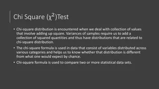
11.1 The Chi-Square Distribution Definition The chi-square distribution has only one parameter called the degrees of freedom (df). The shape of a chi-square distribution curve is bell-shaped and highly skewed to the right for small df (except for df=2 which looks exponential); bell-shaped but more symmetric for large df. The entire chi-square distribution curve lies to the right of the vertical axis. The chi-square distribution assumes nonnegative values: denoted by ?2(read as kie-square ). 3

Three Chi-Square Distribution Curves ?? 2 is peak; ??is mean; the median is somewhere in between. 4

Practice Which of the following is false? As the df increases, (a) the center of the 2 distribution increases as well (b) the variability of the 2 distribution increases as well (c) the shape of the 2 distribution becomes more skewed (less like a normal)

Practice Which of the following is false? As the df increases, (a) the center of the 2 distribution increases as well (b) the variability of the 2 distribution increases as well (c) the shape of the 2 distribution becomes more skewed (less like a normal)

Example of ?2: input of right probability Find the value of ?2 for 7 degrees of freedom and an area of 0.10 in the right tail of the distribution curve. Observe that the area under the pdf in a ?2 distribution is right-tailed. 7

Example of ?2: input of left probability Find the value of ?2 for 12 degrees of freedom and an area of 0.05 in the left tail of the distribution curve. Recall that the area under the ?2 distribution is right tailed. In order to find left-tail area, we should calculate left tail = 1 ??? ? ???? 8

11.2 A Goodness-of-Fit Test Definition An experiment with the following characteristics is called a multinomial experiment. 1. The experiment consists of n identical trials (repetitions). 2. Each trial results in one of k possible outcomes (or categories), where k > 2. 3. The trials are independent. 4. The probabilities of the various outcomes remain constant for each trial. 9

Observed and Expected Frequencies Definition The frequencies obtained from the performance of an experiment are the observed frequencies (denoted by O). The expected frequencies (denoted by E), are those that we expect to obtain if ?0 is true. The expected frequency for a category is obtained as E = ?? where: n is sample size; p is probability an element belongs to category if ?0 is true. 10

Test Statistic for a Goodness-of-Fit Test and its The test statistic for a goodness-of-fit test is value is calculated as 2 ( ) 2 E O E = 2 where O = observed frequency for a category E = expected frequency for a category = np A chi-square goodness-of-fit test: always right-tailed! 11

Conditions for the chi-square test 1. Independence: Each case that contributes a count to the table must be independent of all the other cases in the table. 2. Sample size: Each particular scenario (i.e. cell) must have at least 5 expected cases. 3. df > 1: Degrees of freedom must be greater than 1. Failing to check conditions may unintentionally affect test's error rates.

ATM usage by (work) day A bank has an ATM installed inside a bank, and it is available to customers only from 7 AM to 6 PM Monday - Friday. The manager wants to investigate if the percentage of transactions made on this ATM is the same for each day. In one week, she counts the number of transactions made on this ATM on each of the 5 days. The information she obtains is: Day # of users Monday 253 Tuesday 197 Wednesday 204 Thursday Friday 297 267 At the 1% level of significance, test whether we can reject ?0: # of people who use ATM each of 5 days is the same Assume that this week is typical (not during a holiday season). 13

ATM usage by (work) day: Solution (1 of 3) Step 1: : :At least two of the five proportions are not equal to .20 H Step 2: There are 5 categories: 5 days of ATM usage. = = = = = .20 H p p p p p 0 1 2 3 4 5 1 Step 3: Area in the right tail = = .01 k = number of categories = 5 df = k 1 = 5 1 = 4 The critical value is: ????? = 13.277 (from chart) 2 14

ATM usage by (work) day: Solution (2 of 3) Observed Frequency O 253 197 204 279 267 n = 1200 Expected Frequency E = np 1200(.20) = 240 1200(.20) = 240 1200(.20) = 240 1200(.20) = 240 1200(.20) = 240 ( ) 2 E O E Category (Day) Monday Tuesday Wednesday Thursday Friday p (O E) 13 43 36 39 27 (O minus E) squared 169 1849 1246 1521 729 (O minus E) squared over E(O minus E) squared over E .704 7.704 5.400 6.338 3.038 Sum =23.184 .20 .20 .20 .20 .20 ( ) 2 O E Blank Blank Blank Blank Blank Step 4: From the table: ( 2 = E M T W Th F Total Expected (as %) 20% 20% 20% 20% 20% Observed 253 Expected (as f) 240 (O-E)^2/E 0.7 1 ) 2 O E 197 240 7.7 204 240 5.4 6.34 3.04 279 240 267 240 1200 1200 23.183 = 23.184 The Excel table has been done horizontally rather than vertically & is live! 15

ATM usage by (work) day: Solution (3 of 3) Step 5: The value of the test statistic the critical value of = 23.184 is larger than 2 = 13.277. 2 It falls in the rejection region. Hence, we reject the null hypothesis. We state that the number of persons who use this ATM is not the same for the 5 days of the week. It looks like usage drops off towards the beginning of the week and picks up as the weekend gets closer. 16

Example 11-4 (1 of 2) In a Gallup poll conducted April 3 6, 2014, Americans aged 18 and older were asked if upper-income people were paying their fair share in federal taxes, paying too much or paying too little. Of the respondents, 61% said too little, 24% said fair share, 13% said too much, and 2% had no opinion (gallup.com). Assume that these percentages hold true for the 2014 population of Americans aged 18 and older. Recently, 1000 randomly selected Americans aged 18 and older were asked the same question. The table on the next slide lists the number of Americans in this sample who belonged to each response. 17

Example 11-4 (2 of 2) Response Frequency Too Little 581 Fair Share 256 Too Much 138 No Opinion 25 Test at a 2.5% level of significance whether the current distribution of opinions is different from that for 2014. Step 1: H0 : The current percentage distribution of opinions is the same as for 2014. H1 : The current percentage distribution of opinions is different from that for 2014. 18

Example 11-4 (3 of 2) Step 2: There are 4 categories Multinomial experiment We use the chi-square distribution to make this test. Step 3: Area in the right tail = = .025 k = number of categories = 4 df = k 1 = 4 1 = 3 The critical value of = 9.348. 2 19

Table 11.4 Calculating the Value of the Test Statistic Observed Frequency O 581 256 138 25 n = 1000 Expected Frequency E = np 1000(.61) = 610 1000(.24) = 240 1000(.13) = 130 1000(.02) = 20 Blank ( ) 2 E O E Category (Response) Too little Fair share Too much No opinion Blank ( ) 2 O E p (O E) 29 16 (O minus E) squared 841 256 64 25 Blank Sum = 4.188 (O minus E) squared over E 1.379 1.067 .492 1.250 .61 .24 .13 .02 8 5 Blank Blank 20

Example 11-4: Solution (4 of 5) Step 4: All the required calculations to find the value of the test statistic are shown in Table 11.4. 2 ( ) 2 E O E = = 4.188 2 21

Example 11-4: Solution (5 of 5) Step 5: The value of the test statistic the critical value of = 4.188 is smaller than 2 = 9.348 2 It falls in the nonrejection region. Hence, we fail to reject the null hypothesis. We state that the current percentage distribution of opinions is the same as for 2014. 22

Weldon's dice Walter Frank Raphael Weldon (1860 - 1906), was an English evolutionary biologist and a founder of biometry. He was a founding editor of Biometrika, with Francis Galton and Karl Pearson. In 1894, he rolled 12 dice 26,306 times, and recorded #of 5s or 6s He observed that 5s or 6s occurred more often than expected. Pearson hypothesized that this was due to construction of dice: inexpensive dice have hollowed-out pips; the face with 6 pips is lighter than its opposing face, which has only 1 pip (opposing faces sum to 7). (which he considered to be a success ).

Labby's dice In 2009, Zacariah Labby (U of Chicago), repeated Weldon's experiment using a homemade dice-throwing, pip counting machine. www.youtube.com/watch?v=95EErdouO2w The rolling-imaging process took about 20 seconds per roll. Each day there were ~150 images to process manually. At this rate Weldon's experiment was repeated in a little more than six full days. galton.uchicago.edu/about/docs/labby09dice.pdf

Labby's dice (cont.) Labby did not actually observe the same phenomenon that Weldon observed (higher frequency of 5s and 6s). Automation allowed Labby to collect more data than Weldon did in 1894. Instead of recording "successes" and "failures", Labby recorded the individual number of pips on each die.

Expected counts Labby rolled 12 dice 26,306 times. If each side is equally likely to come up, how many 1s, 2s, ..., 6s would he expect to have observed? (a)1/6 (b)12/6 (c)26,306 / 6 (d)12 x 26,306 / 6

Expected counts Labby rolled 12 dice 26,306 times. If each side is equally likely to come up, how many 1s, 2s, ..., 6s would he expect to have observed? (a)1/6 (b)12 / 6 (c)26,306 / 6 (d)12 x 26,306 / 6 = 52,612

Summarizing Labby's results The table below shows the observed and expected counts from Labby's experiment. At a first glance, does there appear to be an inconsistency between the observed and expected counts.

Labby's dice (cont) The research question is: Do these data provide convincing evidence of an inconsistency between the observed and expected counts? The hypotheses are: H0: There is no inconsistency between the observed and the expected counts. (The observed counts follow the same distribution as the expected counts.) H1: There is an inconsistency between the observed and the expected counts. (The observed counts do not follow the same distribution as the expected counts, i.e., there is a bias in which side comes up on the roll of a die.) We calculate a test statistic of 2= 24.67. ?? = ? 1 = 6 1 = 5

Finding a p-value for a chi-square test The p-value for a chi-square test is defined as the tail area abovethe calculated test statistic.

Conclusion of the hypothesis test We calculated a p-value less than 0.001. At 5% significance level, what is the conclusion of the hypothesis test? (a) Reject H0, the data provide convincing evidence that the dice are fair. (b)Reject H0, the data provide convincing evidence that the dice are biased. (c) Fail to reject H0, data provide convincing evidence that the dice are fair. (d)Fail to reject H0, data provide convincing evidence that dice are biased.

Conclusion of the hypothesis test We calculated a p-value less than 0.001. At 5% significance level, what is the conclusion of the hypothesis test? (a) Reject H0, the data provide convincing evidence that the dice are fair. (b)Reject H0, data provide convincing evidence that the dice are biased. (c) Fail to reject H0, data provide convincing evidence that the dice are fair. (d)Fail to reject H0, data provide convincing evidence that dice are biased.

Turns out... The 1-6 axis is consistently shorter than the other two (2-5 and 3-4), thereby supporting the hypothesis that the faces with one and six pips are larger than the other faces. Pearson's claim that 5s and 6s appear more often due to the carved-out pips is not supported by these data. Dice used in casinos have flush faces, where the pips are filled in with a plastic of the same density as the surrounding material and are precisely balanced.

Recap: p-value for a chi-square test The p-value for a chi-square test is defined as the tail area above the calculated test statistic. This is because the test statistic is always positive, and a higher test statistic means a stronger deviation from the null hypothesis.