Classical Mechanics and Mathematical Methods: Lecture 8 - Calculus of Variation

This content provides information on Lecture 8 focusing on the calculus of variation, including topics like the Brachistochrone problem, calculus of variation with constraints, and its applications in classical mechanics. Questions from students are addressed regarding assignments, integral equations, and concepts like the Euler-Lagrange equation.

• Classical Mechanics
• Mathematical Methods
• Calculus of Variation
• Lecture
• Classical Physics

beaubien_j Follow

Uploaded on Feb 27, 2025 | 0 Views

Download Presentation

Please find below an Image/Link to download the presentation.

The content on the website is provided AS IS for your information and personal use only. It may not be sold, licensed, or shared on other websites without obtaining consent from the author.If you encounter any issues during the download, it is possible that the publisher has removed the file from their server.

You are allowed to download the files provided on this website for personal or commercial use, subject to the condition that they are used lawfully. All files are the property of their respective owners.

The content on the website is provided AS IS for your information and personal use only. It may not be sold, licensed, or shared on other websites without obtaining consent from the author.

Presentation Transcript

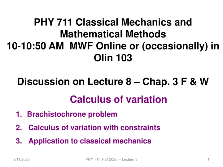
1. PHY 711 Classical Mechanics and Mathematical Methods 10-10:50 AM MWF Online or (occasionally) in Olin 103 Discussion on Lecture 8 Chap. 3 F & W Calculus of variation 1. Brachistochrone problem 2. Calculus of variation with constraints 3. Application to classical mechanics 9/11/2020 PHY 711 Fall 2020 -- Lecture 8 1

2. Schedule for weekly one-on-one meetings Nick 11 AM Monday (ED/ST) Tim 9 AM Tuesday Bamidele 7 PM Tuesday Zhi 9 PM Tuesday Jeanette 11 AM Friday Derek 12 PM Friday 9/11/2020 PHY 711 Fall 2020 -- Lecture 8 2

3. Your questions From Nick 1. Can you go over the directions for the next assignment? I'm a bit confused as to what you're asking for in parts a,b. 2. Can you discuss a little more the setup for the T= integral equation at the top of slide 7? Why are we integrating ds/v? 3. Also, in the development of the alternative Euler-Lagrange, we get this relationship: Please explain. From Tim 1. On slide 8 you give the quantity inside the brackets as equal to K = 2a. Did you just do this to make it easier, because in the previous process it would have turned out to be 1/k^2. From Gao 1. About lecture #8, what does W=E+ L stand for (15th page of note)? Thank you. 9/11/2020 PHY 711 Fall 2020 -- Lecture 8 3

4. 9/11/2020 PHY 711 Fall 2020 -- Lecture 8 4

5. 9/11/2020 PHY 711 Fall 2020 -- Lecture 8 5

6. Your question -- please explain HW 6 a little better. Suppose that we have a generalized coordinate ( ) that varies with time and a ( ) ), ( ); = q t t q t t dq dt function that has the dependences ( ), ( ); t t . As an example, suppose f q t df dt = / 2 2 t that ( ) and ( Evaluate in two different ways q t e f q t qq t for (d) and (c). You should get the same answer. For parts (a) and (b) you are asked to take two derivatives in different orders. The surprising. results may be 9/11/2020 PHY 711 Fall 2020 -- Lecture 8 6

7. dy Review for : ( ), , , f y x x dx x dy f x necessary a condition extremize to : f y(x), ,x dx dx i f d f dy = 0 Euler-Lagrange equation ( ) / y dx dy dx dy , , x x y dx dy Note that for ( ), , , f y x x dx df f dy f d f = + + ( ) / dx y dx dy dx dx dx x d f dy f d dy f dy = + + ( ) ( ) / / dx dy dx dx dy dx dx dx x d f f Alternate Euler-Lagrange equation = f ( ) / dx dy dx dx x 9/11/2020 PHY 711 Fall 2020 -- Lecture 8 7

8. Your question Also, in the development of the alternative Euler-Lagrange, we get this relationship: Please explain. Suppose that ( ) is the function that extremizes the integral y x x dy dx f . We then "derived" the Euler-Lagrange relation ,x dx = f y(x), x i f y d dx f f y d dx f = 0 ( ) ( ) / / dy dx dy dx dy dx dy dx , , x x , , x y x y 9/11/2020 PHY 711 Fall 2020 -- Lecture 8 8

9. A few more steps -- dy dy Note that for ( ), , , f y x x dx df f dy f d f = + + ( ) / dx y dx dy dx dx dx x d f dy f d dy f dy = + + ( ) ( ) / / dx dy dx dx dy dx dx dx x d f f = f ( ) / dx dy dx dx x 9/11/2020 PHY 711 Fall 2020 -- Lecture 8 9

10. Brachistochrone problem: (solved by Newton in 1696) http://mathworld.wolfram.com/BrachistochroneProblem.html A particle of weight mg travels frictionlessly down a path of shape y(x). What is the shape of the path y(x) that minimizes the travel time from y(0)=0 to y( )=- ? Note that the increment of travel time path length is speed ds v = dt 1 2 = + 2 E mv mgy = With the choice of initial conditions, 0 E 9/11/2020 PHY 711 Fall 2020 -- Lecture 8 10

11. Vote for your favorite path x y Which gives the shortest time? a. Green b. Red c. Blue 9/11/2020 PHY 711 Fall 2020 -- Lecture 8 11

12. 2 dy dx gy + 1 x y x f f f ds v = = = 2 because 1 2 T dx mv mgy 2 i i x y x i 2 dy dx y + 1 dy dx Note that for the original form of Euler-Lagrange equation: = ( ), y x , f x d dx f dy f y d dx f = = 0 f 0, ( ) ( ) / / dy dx dx dy dx dy dx , x , x y differential equation is more complicated: 1 d dx 2 dy dx y dy dx = 0 + 1 1 2 d dx 2 dy dx = 0 + 1 y 3 2 dy dx + 1 y 9/11/2020 PHY 711 Fall 2020 -- Lecture 8 12

13. 2 dy + 1 dy dx = ( ), , f y x x dx y d f dy f = f ( ) / dx dy dx dx x 2 1 d dy = + = 0 1 2 y K a dx dx 2 dy + 1 y dx Question why this choice? Answer because the answer will be more beautiful. (Be sure that was not my cleverness.) 9/11/2020 PHY 711 Fall 2020 -- Lecture 8 13

14. 2 dy ( ) d + = = = a cos a 2 1 2 2 y K a Let 2 dy sin cos 1 y a a dx 2 2 2 2 sin = = dx 2 dy a 2 a = 1 1 1 dx y 2 2 2 sin y a dy 2 = dx ( ) ( ) 0 = d = 1 cos ' ' sin x a a a 1 y Parametric equations for Brachistochrone: ( ( cos = a y ) = sin x a ) 1 9/11/2020 PHY 711 Fall 2020 -- Lecture 8 14

15. Parametric plot -- plot([theta-sin(theta), cos(theta)-1, theta = 0 .. Pi]) y x 9/11/2020 PHY 711 Fall 2020 -- Lecture 8 15

16. Checking the results 2 dy dx gy + 1 x y x ds v f f f = = T dx 2 i i x y x i T=infinite T=5.2668 T=4.4429 1 (units of ) (2 ) g 9/11/2020 PHY 711 Fall 2020 -- Lecture 8 16

17. Summary of the method of calculus of variation -- Consider a family of functions ( ), with the end points ( ) and ( ) and an integral function i i f f y x y y x y = = y x x f dy dx dy dx ( ), y x , = ( ), y x ; . I x f x dx x i dy dx Find the function ( ) which extremizes y x ( ), y x , . I x = 0 Euler-Lagrange equation: I f y d dx f = 0 for all x x x ( ) i f / dy dx dy dx , x , x y 9/11/2020 PHY 711 Fall 2020 -- Lecture 8 17

18. Euler-Lagrange equation: f y d dx f = 0 ( ) / dy dx dy dx , x , x y Alternate Euler-Lagrange equation: d dx f dy f x = f ( ) / dy dx dx 9/11/2020 PHY 711 Fall 2020 -- Lecture 8 18

19. Another example optimization problem: Determine the shape y(x) of a rope of length L and mass density hanging between two points x1 y1 x2 y2 9/11/2020 PHY 711 Fall 2020 -- Lecture 8 19

20. Example from internet -- 9/11/2020 PHY 711 Fall 2020 -- Lecture 8 20

21. Potential energy of hanging rope : 2 x dy 2 = + : 1 E g y dx dx x of 1 Length rope 2 x dy 2 = + 1 L dx dx x 1 composite a Define function t minimize o : + W E L Lagrange multiplier 9/11/2020 PHY 711 Fall 2020 -- Lecture 8 21

22. Your question -- what does W=E+L stand for? Comment -- W does not have an obvious physical interpretation = = + But W 0 for fixed E L is a very clever mathematical trick to help solve the minimization and constraint at the same time. 9/11/2020 PHY 711 Fall 2020 -- Lecture 8 22

23. 2 x dy 2 ( ) = + + 1 W gy dx dx x 1 2 dy dy ( ) = + + , 1 f y gy dx dx d f dy f = f ( ) / dx dy dx dx x 2 dy 2 dy dx ( ) + + = 1 gy K dx 2 dy + 1 dx 9/11/2020 PHY 711 Fall 2020 -- Lecture 8 23

24. 2 dy 2 dy dx ( ) + + = 1 gy K dx 2 dy + 1 dx 1 ( ) + = gy K 2 dy + 1 dx / 1 x a = + ( ) cosh y x K g K g 9/11/2020 PHY 711 Fall 2020 -- Lecture 8 24

25. / 1 x a , = + ( ) cosh y x K g K g Integratio constants n : , K a = Constraint : s ( ) y x y 1 1 = ( ) y x y 2 2 2 x dy 2 + = 1 dx L dx x 1 9/11/2020 PHY 711 Fall 2020 -- Lecture 8 25

26. Summary of results For the class of problems where we need to perform an extremization on an integral form: x f dy dx = = ( ), y x , 0 I f x dx I x i A necessary condition is the Euler-Lagrange equations: = f y d dx f = 0 ( ) / dy dx d dx f dy f x f ( ) / dy dx dx 9/11/2020 PHY 711 Fall 2020 -- Lecture 8 26

27. Application to particle dynamics (time) (generalized coordinate) (Lagrangian) or (action) A S dq q dt x y f I t q L Denote: t 2 ( ) = , ; A L q q t dt t 1 9/11/2020 PHY 711 Fall 2020 -- Lecture 8 27

28. Application to particle dynamics Hamilton s principle states that the dynamical trajectory of a system is given by the path that extremizes the action integral ( , ; t t t dy dt 2 2 ) = , ; A L q q t dt L y t dt t 1 1 Simple example: vertical trajectory of particle of mass m subject to constant downward acceleration a=-g. 2 d y dt y t = Newton's formulation: m mg 2 = + 2 Resultant trajectory: ( ) Lagrangian for this case: y vt gt 1 2 i i 2 1 2 dy dt = L m mgy 9/11/2020 PHY 711 Fall 2020 -- Lecture 8 28

29. http://www-history.mcs.st-and.ac.uk/Biographies/Hamilton.htmlhttp://www-history.mcs.st-and.ac.uk/Biographies/Hamilton.html 9/11/2020 PHY 711 Fall 2020 -- Lecture 8 29

30. https://irishpostalheritagegpo.wordpress.com/2017/06/08/william-rowan-hamilton-irish-mathematician-and-scientist/https://irishpostalheritagegpo.wordpress.com/2017/06/08/william-rowan-hamilton-irish-mathematician-and-scientist/ 9/11/2020 PHY 711 Fall 2020 -- Lecture 8 30

31. Now consider t Lagrangian he defined to be : dy ( ), , L y t t T U dt Potential energy Kinetic energy In our example: 2 1 2 dy dt dy dt = ( ), y t , L t T U m mgy Hamilton's principle states: t f dy dt ( ), y t , is minimized for physical ( ): S L t dt y t t i 9/11/2020 PHY 711 Fall 2020 -- Lecture 8 31

32. Condition for minimizing the action in example: t 2 1 2 f dy dt S m mgy dt t i Euler-Lagrange relations: L d L y dt y d mg dt d dy dt dt = 0 = 0 my = + 2 ( ) y t y v t gt 1 = g i i 2 9/11/2020 PHY 711 Fall 2020 -- Lecture 8 32

33. Check: t 2 1 2 f dy dt S m mgy dt t i = = = = 2 Assume 0, ; , 0 1 2 t y h gT t T y i i f f ( ) = = 2 Trial trajectories: ( ) 1 / 1 2 1 2 y t gT t T h gTt 1 ( ( ) ) ( ) = = 2 2 2 2 1 / 1 2 1 2 y t gT t T h gt 2 ( ) = = 2 3 3 3 1 / / 1 2 1 2 y t gT t T h gt T 3 Maple says: = = = 2 3 0.125 S mg T 1 2 3 0.167 S mg T 2 2 3 0.150 S mg T 3 9/11/2020 PHY 711 Fall 2020 -- Lecture 8 33