Explore the intricacies of closed-loop motion control systems in electric drives, focusing on torque, speed, and position precision. Learn how vector control enhances efficiency and simplifies control strategies for various motor types. Dive into the cascaded motion control method and grasp the essentials of torque loop design for PM DC brush motors. Delve into practical examples and numerical analysis to deepen your understanding of motion control principles in electric drives.
Please find below an Image/Link to download the presentation.
The content on the website is provided AS IS for your information and personal use only. It may not be sold, licensed, or shared on other websites without obtaining consent from the author. If you encounter any issues during the download, it is possible that the publisher has removed the file from their server.
You are allowed to download the files provided on this website for personal or commercial use, subject to the condition that they are used lawfully. All files are the property of their respective owners.
The content on the website is provided AS IS for your information and personal use only. It may not be sold, licensed, or shared on other websites without obtaining consent from the author.
7. CLOSED LOOP MOTION CONTROL IN ELECTRIC DRIVES 7.1. INTRODUCTION By motion control we mean torque, speed or position control. Motion control systems are characterized by precision, response quickness and immunity to parameter detuning, torque and inertia perturbations and energy conversion rates. Motion control through electric motors and power electronic converters (P.E.Cs) may be approached by the theory and practice of linear and nonlinear, continuous or discrete control systems. . PM d.c. - brush motors are characterized by a low electrical time constant e = L / R of a few miliseconds or less. The armature (torque) current is fully decoupled from the PM field because of the orthogonality of the armature and PM fields, both at standstill and for any rotor speed. Electric Drives 2
As shown in later chapters, vector control of a.c. motors does also decoupled flux and torque control if the orientation of the flux linkage is kept constant. Consequently vector controlled a.c. motors are similar to d.c. brush motors and thus the application of various motion control systems to the d.c. motor holds notable generality while also eliminates the necessity of a separate chapter on closed loop control of brushless motors. 7.2. THE CASCADED MOTION CONTROL The PM d.c. - brush motor equations are: di V PM (7.1) = + + Ri L r dt Figure 7.1. Typical cascaded motion control Electric Drives 3
d = r J T T L (7.2) e dt d = (7.3) r r dt = T I (7.4) e PM 7.2.1. The torque loop For constant (or zero) load torque the PM d.c. brush motor current / voltage transfer function, from (7.1) - (7.4), becomes: ( ) ( ) ( s V s + i s ( ) s = = em H )R V (7.5) + 2 s s 1 em e em JR = where (7.6) em 2 PM Electric Drives 4
Figure 7.2. PI torque loop for a PM d.c. brush motor In what follows we are using the critical frequency c and phase margin c contraints for the open - loop transfer function A(s) of the system on figure 7.2.: ( ) R s si ( ) + K 1 s K K K + s + (7.7) = si si C T I em A s 2 s s 1 em e em The critical frequency c should be high - up to 1...2 kHz - to provide fast torque (current) control. Electric Drives 5
Let us have as a numerical example a PM d.c. brush motor with the data: Vn = 110V, Pn = 2kW, nn = 1800rpm, R = 1 , L = 20mH, KT = 1.1Nm/A, em = 0.1 sec., KC = 25V/V, Ki = 0.5V/A, critical frequency fc = 500Hz, and the phase margin c = 47 . The phase margin c of A(s) from (7.7), for the critical frequency c = 2 fc, is: + = c Arg 180 ( ) = 0 A j c 2 si (7.8) ( ) = + 0 1 1 c em 180 tan tan c 1 c em e Consequently: 500 1 . 0 2 ( ) tan ( (7.9) = + + = 1 0 0 1 0 180 47 tan 46 ) c si 2 500 1 . 0 . 0 1 2 02 And thus: 0 tan 46 500 3075 . 0 (7.10) = = ms si 2 Electric Drives 6
The gain of the torque controller Ksi may be calculated from the known condition: j A ( ) c = 1 (7.11) ( 10 ) ( 1 + ) 2 2 1 . 0 + . 0 3 3 6 2 3075 . 0 10 1 10 1 . 0 01 = = Finally: K . 2 205 si 1 . 1 5 . 0 1 . 0 2 25 1 . 0 965 7.2.2. The speed loop (7.12) Figure 7.3. Speed control with torque (current) inner loop Electric Drives 7
The block diagram on figure 7.3. may be restructured as in figure 7.4. where K is the gain of the speed sensor. Figure 7.4. Simplified speed loop block diagram For the speed loop design we may proceed as above for the torque loop, but with a critical frequency fc = 100Hz and a phase margin c = 60 with K = 0.057 V sec/rad. The final results are: s = 2.87ms and Ks = 2.897 103. The amplification Ks is rather high but the phase margin is ample and produces a reasonably low overshoot and well damped oscillatory response. Electric Drives 8
7.2.3. Digital position control The basic configuration of digital position control system is shown in figure 7.5. Figure 7.5. Basic digital position control system Suppose only an 8 bit DAC with Vd = 10V is used. Consequently its amplification Kd is: 2 2 2 V n 20 20 = = = d K V / pulse (7.13) d 8 256 The amplification of the encoder Kp is: 4 N = Kp pulse / rad (7.14) 2 Electric Drives 9
The position control is performed in a DSP with the discretization period of T. The position error (KT) is: ( ) ( KT KT r = (7.15) ) ( ) * KT r The position controller filters this error to produce the command Y(KT) which is periodically applied through the DAC: Y K V d C = ) (7.16) ( KT The command voltage Vc is kept constant during the discretization period T, the effect being known as ZOH. The digital filter may be expressed by finite difference equations of the type [2]: ( ) ( ) ( ( ) ) = Y KT 2 KT K 1 T (7.17) Z - transform may be used to model (7.17). The Z transform shifting property is: ( ) ( ) Z f Z m K Y ( ) K ( ) Z (7.18) m with f f Electric Drives 10
Consequently (7.17) becomes: The D(Z) is thus: ( ) Z ( ) Z ( ) ( ) Z ( ) Z (7.19) = 1 Y 2 Z Y Z 2 Z 1 ( ) Z s (7.20) = = D Z K ( ) ( ) C V ( ) s s (7.21) = = s c M ( ) + s 1 s K em T The data for this new numerical example are: KT = 0.1Nm/A, R = 1 , L = 0H, J = 10-3kgm2, Kc = 5V/V with the critical frequency c = 125rad/sec. and the phase margin cp = 45o. The problem may be solved adopting a continual filter (controller) and finally "translating" it into a discrete form. The motor converter transfer function M(s) is: 3 50 RJ 1 10 ( ) s + ; (7.22) = = = = M s 1 . 0 ( ) em 1 . 0 2 2 s 1 s 1 . 0 K T Electric Drives 11
The DAC amplification is Kd = 10/128 (8 bit). The encoder produces N = 500 pulses / revolution which provides in fact 4N = 2000 pulses / revolution, and has the amplification Kp: 2 2 4 N 2000 (7.23) = = = Kp 318 pulses / rad The discretisation (sampling) time is T = 10-3 sec. Thus the ZOH transfer function is: The various transfer functions in figure 7.5 are united in a unique transfer function H(s): or: ( ) ( 1 s + sT ( ) s 4 5 10 = s ZOH e e 2 (7.24) ( ) s ( ) s ( ) s = H K K ZOH M (7.25) d p 4 5 10 s 1242 8 e = H s (7.26) ) 1 . 0 s The phase angle of H(s) for c is: 0 T 180 ( 1 . 0 ) = = 179 0 1 0 2 (7.27) c 90 tan 125 H Electric Drives 12
To produce a phase margin c of 45 the digital filter D(A) has to produce a phase anticipation D of 44 . A tentative D(s) lead - lag filter is: ( ) s + s = 1 G s K + phase angle D is: The maximum anticipation is obtained for c = ( 1 2)0.5. The filter (7.28) 2 (7.29) = 1 1 c c tan tan D 1 2 with c = 125 rad./sec. and D = 44 , 1 = 53.3 rad./sec. and 2 = 293.15rad/sec. Finally the amplification K of G(s) is obtained from the condition that the amplitude of open loop transfer function of the system H(s) G(s) be equal to unity for critical frequency. With the above data K = 2.96. Electric Drives 13
To discretise the G(s) transfer function, the correspondence between Z and s is considered: 1 Z T + 2 Z 1 = = s 2000 + Z 1 Z 1 Consequently G(Z) is: (7.30) ( ) ( ) Z Z . 0 947 Y Z ( ) Z = = G 265 Z (7.31) . 0 744 or: ( ) Z ( ) Z ( ) Z ( ) Z = 1 1 Y . 0 744 Z Y . 2 65 . 2 51 Z (7.32) Finally the output of the digital filter Y(k) is: ( ) k ( ) ( ) k ( ) 1 = + (7.33) Y . 0 744 Y k 1 . 2 65 . 2 51 k Electric Drives 14
7.2.4 Positioning precision It is known that the positioning precision is influenced by the friction torque. Let us consider a friction torque Tf = 0.05Nm. The speed is small around the target position and thus the motion induced voltage of the motor may be neglected: T R I R V T . 0 1 05 = = = = f 5 . 0 V K 1 . 0 The command voltage of the static power converter Vc is: (7.34) V 5 . 0 = = = V . 0 05 V c The DAC input Nc is: (7.35) K 5 c V . 0 05 = = = c N . 0 64 pulses c 10 K 128 (7.36) d Electric Drives 15
The gain of the digital filter Ko is obtained for Z = 1: 1 . 0 94 = = K0 . 2 65 . 0 548 1 . 0 7441 Consequently the input of the digital filter Ne is: (7.37) N . 0 64 = = pulses 33 . 1 = c N e K . 0 548 The closest integer is Nei = 2 pulses and thus the position error r caused by the above friction torque is: 0 e r N 4 (7.38) 0 N 360 2 360 = = = 0 . 0 36 2000 The precision of positioning may be improved through diverse methods such as the increasing of the encoder number of pulses per revolution N or by a feedforward signal proportional to the torque perturbation. Optical encoders with up to 20,000 pulses / revolution are available today. Industrial position controllers in digital implementation are, in general, of P type but contain a speed feedword signal and an inner PI speed loop besides the torque loop (figure 7.6) [4]. (7.39) Electric Drives 16
Figure 7.6. Standard digital position control system with inner speed loop ^ ^ * It should be noticed that both and - estimated reference speed and actual speed - are calculated through the position time derivative and thus contain noise and errors.In general such a controller responds well to slow dynamics commands, well beyond the frequency of the position controller (0.5 to 10Hz). For this reason, in order to follow correctly the targeted position during transients, in the presence of torque and inertia changes, state space control is used where the speed and acceleration are estimated adequately from the measured position. r r Electric Drives 17
7.3. STATE - SPACE MOTION CONTROL In such systems there is a separation of position tracking commands from those related to perturbation rejection. To yield zero position tracking errors a positive torque reaction is used. That does not affect the stability to perturbations but poses problems to torque dynamics and estimation precision (figure 7.7). ( ) k ( ) k 1 ^ (7.40) = r r r T Electric Drives 18


 becomes:")
. The encoder")

 transfer function, the correspondence")