Cluster Analysis in Multivariate Statistics

This content delves into various multivariate statistical techniques such as PCA, correspondence analysis, canonical correlation, discriminant function analysis, cluster analysis, and MANOVA. It includes examples of using cluster analysis to group data points using hierarchical clustering and k-means clustering methods. The determination of the optimal number of clusters is explored through within-cluster sum of squares analysis. Xuhua Xia presentations are referenced throughout the content to illustrate the application of these techniques.

• Multivariate Statistics
• Cluster Analysis
• PCA
• Hierarchical Clustering
• K-means Clustering

jolivette_s Follow

Uploaded on Apr 17, 2025 | 0 Views

Download Presentation

Please find below an Image/Link to download the presentation.

The content on the website is provided AS IS for your information and personal use only. It may not be sold, licensed, or shared on other websites without obtaining consent from the author.If you encounter any issues during the download, it is possible that the publisher has removed the file from their server.

You are allowed to download the files provided on this website for personal or commercial use, subject to the condition that they are used lawfully. All files are the property of their respective owners.

The content on the website is provided AS IS for your information and personal use only. It may not be sold, licensed, or shared on other websites without obtaining consent from the author.

Presentation Transcript

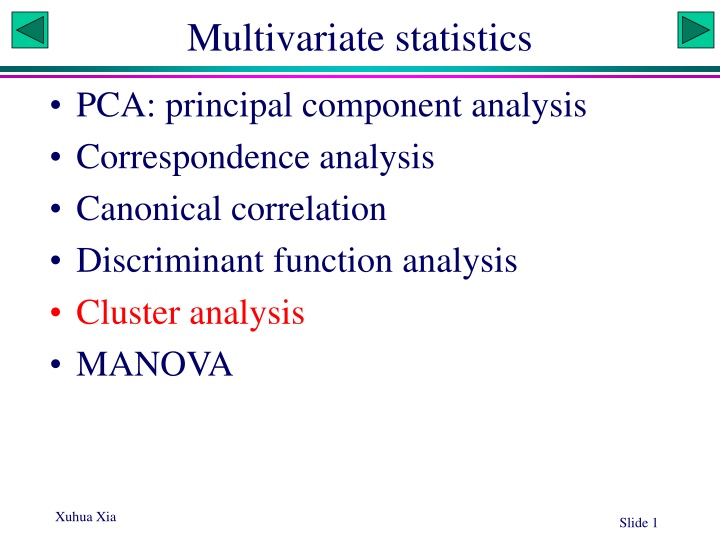
1. Multivariate statistics PCA: principal component analysis Correspondence analysis Canonical correlation Discriminant function analysis Cluster analysis MANOVA Xuhua Xia Slide 1

2. Cluster analysisPCA md<- read.fwf("http://dambe.bio.uottawa.ca/teach/bio8102_download/Crime.txt ", c(14,6,5,6,6,7,7,6), header=T) nd<-scale(md[,2:8]) d<-dist(nd,method="euclidean") # other distances:, "maximum|manhattan|Canberra|binary|minkowski" hc<-hclust(d) sLabel<-substr(md$STATE,1,4) plot(hc,labels=sLabel) rect.hclust(hc, k=4, border="red") Slide 2

3. Cluster plot Cluster Dendrogram 8 6 Height 4 New Alas Mass 2 Flor Ariz Rhod Texa Nort Miss Sout New Neva Cali West Colo Dela Hawa Kent Penn 0 Alab Loui Illi Nort Sout Mary Mich Arka Okla Nebr New Conn Indi Kans Virg Minn Utah Geor Tenn New Miss Ohio Verm Main Idah Wash Oreg Mont Wyom Wisc Iowa d Xuhua Xia Slide 3 hclust (*, "complete")

4. Group into clusters Cluster Dendrogram 8 6 Height 4 New Alas Mass 2 Flor Ariz Rhod Texa Nort Miss Sout New Neva Cali West Colo Dela Hawa Kent Penn 0 Alab Loui Illi Nort Sout Mary Mich Arka Okla Nebr New Conn Indi Kans Virg Minn Utah Geor Tenn New Miss Ohio Verm Main Idah Wash Oreg Mont Wyom Wisc Iowa Xuhua Xia Slide 4 d hclust (*, "complete")

5. Determining number of clusters (k) # Rationale: plot within-cluster sum of squares over k, with k=2:15 # wss: within-group sum of squares # apply(nd,2,var): calculate variance for each variable; 1|2: variables in # rows|column # sum(apply(nd,2,var)): sum of variance # DF*var = SS wss <- (nrow(nd)-1)*sum(apply(nd,2,var)) # kmeans clustering with 2, 3, , 15 clusters and compute wss for each for (i in 2:15) wss[i] <- sum(kmeans(nd, centers=i)$withinss) plot(1:15, wss, type="b", xlab="Number of Clusters", ylab="Within groups sum of squares") # K-Means Cluster Analysis fit <- kmeans(nd, 5) # 5 cluster solution # get cluster means aggregate(nd,by=list(fit$cluster),FUN=mean) # append cluster assignment nd <- data.frame(nd, fit$cluster) Xuhua Xia Slide 5

6. Number of clusters 350 300 bending of curve Within groups sum of squares 250 200 150 100 50 2 4 6 8 10 12 14 Xuhua Xia Number of Clusters Slide 6