Cointegration in Economics: An Intuitive Explanation
Explore the concept of cointegration in economics using a simple supply and demand model. Learn about equilibrium, dynamics of the system in disequilibrium, and how the system adjusts to reach equilibrium over time.

Uploaded on | 0 Views
Download Presentation

Please find below an Image/Link to download the presentation.
The content on the website is provided AS IS for your information and personal use only. It may not be sold, licensed, or shared on other websites without obtaining consent from the author. If you encounter any issues during the download, it is possible that the publisher has removed the file from their server.
You are allowed to download the files provided on this website for personal or commercial use, subject to the condition that they are used lawfully. All files are the property of their respective owners.
The content on the website is provided AS IS for your information and personal use only. It may not be sold, licensed, or shared on other websites without obtaining consent from the author.
E N D
Presentation Transcript
Cointegration: an intuitive explanation
Consider the simplest economics model; demand & supply There are 3 variables involved: quantity demanded (Qd), quantity supplied (Qs), price (P) By the way, even in the simplest setup, there is no distinction between dependent and independent variables (they all affect and interact with each other), keep this at the back of your head**** What is equilibrium? A certain (unique) price that makes quantity demanded equal to the quantity supplied (Qs = Qd) or Qs Qd =0 Note that there is a linear combination that relates to eqm (1, -1)
Graphically, the point of intersection between the demand and supply curves What happens there? NOTHING, that s why it is called equilibrium Using physics jargon, the system is in equilibrium, all forces cancel each other out, and nothing changes. Hence in eqm: Qs = Qd = P = 0.
How does the system work if it is in disequilibrium? Suppose the price is too high (relatively to the eqm price) Then, we observe excess supply (demand is too low relatively to the supply) The system in order to return to its equilibrium state, starts making some adjustments: The price starts falling, and as this happens, quantity demanded starts increasing, while quantity supplied starts dropping Mathematically, Qs < 0 , Qd > 0, P <0 The exact opposite would happen if the price was too low
So, we observe that the system develops some dynamics, with the variables involved making an adjustment so as the system to reach the eqm The eqm behaves as an attractor (if we are away from eqm, there are forces developed, which make an attempt to bring the system back to equilibrium) So the system might be occasionally (in fact quite often) in disequilibrium, even for quite some time, but if the eqm is meaningful there are will an observed dynamic adjustment towards eqm
Cointegration definition & implications Assume two time series, each of which is I(1) **non-stationary In principle, their linear combination will also be non-stationary If however, there exists a linear combination that is stationary, then the series are cointegrated, and vice versa, If two series are cointegrated, there exists a linear combination of them that is stationary If the series are cointegrated, then there is a long run relationship between them (and vice versa) Hence, their co-behaviour will be such that deviations from their long run relationship should be eliminated
The econometric setup The previous discussion reveals that in a cointegrated system, both short and long run behaviours are involved The long run is captured by the levels of the time series and the eqm relationship they obey The short run is captured by the adjustments the participating variables make in order to bring the system back to eqm All the above are manifested in the Engle-Granger Representation theorem
The Engle-Granger Representation Theorem = + + 1 + + 1 + + ( ) ..... .... X c Y X X Y 1 1 1 1 1 1 t t t x t y t xt = + + 1 + + 1 + + ( ) ..... .... Y c Y X X Y 2 2 1 1 1 1 t t t x t y t yt
Main concepts to be aware of Reaction to disequilibrium Exogeneity Weak exogeneity Short-run Granger Causality Strong Exogeneity
Reaction to disequilibrium The levels appear in the so-called Error Correction Mechanism (ECM), and enter the model with 1-period lag (the system must respond to past deviation from the eqm, if any exists) The s are called Speed-of-Adjustment coefficients and show the speed at which each variable reacts to disequilibrium (in order to bring the system back to eqm) In fact, the inverse of the absolute value ( 1 / abs( ) ) tells you how many periods are needed until a given deviations from eqm is covered E.g if is 0.25, then 1/0.25 = 4, meaning that a given distance from eqm will be cleared in 4 time periods
Weak exogeneity If a variable has an insignificant speed of adjustment coefficient (=0), then this variable does not respond to deviations from eqm Then this variable is WEAKLY EXOGENOUS (it affect the long run relationship, but its NOT affected by it) Can such a thing happen? Note, that at least one of the speed of adjustment parameters must be statistically significant. Why? If all of them were zero, then no variable would respond and therefore, the system would never return to eqm Hence, eqm is not meaningful
(short-run) Granger Causality Recall that the system involves the short-run dynamics (captured by the s of the variables) Each variable is allowed to be affected by two sets of short-run dynamics (lags): its own and symmetrically by the other variable s If a given variable is reacting to the other variable s short-run dynamics, then it is Granger Caused by this variable This is tested by a joint test, where the cross-coefficients of s are set to zero If the hypothesis is not rejected, then there is no Granger Causality
Strong exogeneity If a variable is weakly exogenous (does not respond to disequilibrium) And Is a not Granger Caused in the short-run by any other member of the system, then This variable is STRONGLY EXOGENOUS It is neither affected by the system in the long nor in the short run


 Granger Causality")