Complex Numbers and Algebra: Understanding Phasors and Polar Forms
Dive into the world of complex numbers, phasors, and algebra in electromagnetic wave analysis. Learn about polar forms, Euler's identity, complex conjugates, addition, subtraction, multiplication, division, and square roots of complex numbers. Master the notation and mathematical operations essential for applied electromagnetics.

Download Presentation

Please find below an Image/Link to download the presentation.
The content on the website is provided AS IS for your information and personal use only. It may not be sold, licensed, or shared on other websites without obtaining consent from the author. If you encounter any issues during the download, it is possible that the publisher has removed the file from their server.
You are allowed to download the files provided on this website for personal or commercial use, subject to the condition that they are used lawfully. All files are the property of their respective owners.
The content on the website is provided AS IS for your information and personal use only. It may not be sold, licensed, or shared on other websites without obtaining consent from the author.
E N D
Presentation Transcript
ECE 3317 Applied Electromagnetic Waves Prof. David R. Jackson Fall 2024 Notes 2 Complex Vectors Adapted from notes by Prof. Stuart A. Long 1
Notation Circuit quantities: v(t) is a time-varying function. Note: Handscript SF font is used for time-domain vector quantities. (This font has been placed on Canvas for you.) V is a phasor (complex number). Field quantities: E(t) is a time-varying vector function. E is a phasor vector (complex vector). Ex(t) is a time-varying component of a vector function. Ex is a phasor component of a vector function. Appendix B in the Hayt & Buck book discusses units in some detail. 2
Complex Numbers = a + = j | | c e c j b j = 1 Phase (always in radians) Real part Magnitude Imaginary part Note: a, b, are real. Euler s identity allows us to write the polar form. Euler's identity: Polar form: = + 2 2 c a b = + je cos sin j ( ) Im cos c = + c a jb b ( ) c = + | | cos c sin c j ( ) sin c = = cos a c Re a sin b c Note: The angle is measured positive going counterclockwise. 3
Complex Numbers (cont.) Complex conjugate ( ) = + = 1 j | | c a jb c e 1 1 1 1 ( ) ( ) ( ) * j = = + | = = * 1 | c c a jb a jb c e 1 2 1 1 1 1 1 2 1 Im Im = + c a jb 1 1 1 = a a 2 1 Re 1b = 1 2 1 = b b Re 2 1 1a = = * 1 c c a jb 2 1 1 4
Complex Algebra = = + + = j a | | c jb c e 1 1 1 1 1 c = j | | c a jb e 2 2 2 2 2 Addition + = + + + ( ) ( ) c c a a j b b 1 2 1 2 1 2 Subtraction = + ( ) ( ) c c a a j b b 1 2 1 2 1 2 5
Complex Algebra (cont.) = = + + = j a | | c jb c e 1 1 1 1 1 c e = j | | c a jb 2 2 2 2 2 Multiplication ( )( ) ( )( ) 1 c ( )( ) ( ) ( ) = + + = + + c c a jb a jb 1 2 a a 1 2 bb j a b a b 1 2 1 1 2 2 1 2 2 1 ( + ) = j c c c e 2 1 2 Division ( )( + ) ( ) 2 2 ( 2 2 ) + + + + + + + + a jb a a b jb 1 2 a a jbb j ba b 1 2 a b c c c c a a c c jb jb a a jb jb a a jb jb = = = = 1 1 2 2 2 2 2 2 1 2 1 2 1 1 1 1 1 2 2 a 2 2 2 2 2 2 2 = ( ) j 1 e 1 1 2 2 6
Square Root = j c c e Principal square root of a complex number (denoted by radical sign): ( ) 1/2 = j c c e (the principal branch) ( ) /2 j c e Im b Note: For a positive real number x, the principal square root is positive: c = 4 2 Example: Re a 7
Square Root c e = j c Illustration of principal square root: ( ) /2 j = c c e y Branch cut (line of discontinuity) = /2 j c e j c = 1 x c = 1 = /2 j c e j Here we approach the point c = -1 from above or below the negative real axis (the two red dots). = + Note: Matlab uses the principal square root: 1 j 8
Square Root (cont.) c e = j Property of principal square root: c ( ) /2 j = c c e / 2 / 2 / 2 Examples: = 4 2 c Re 0 + 1 j = = = /2 /4 j j 1 1 j e e 2 9
Square Root (cont.) = j c c e General square root of a complex number: ( ( ) 1/2 = 1/2 j c c e Denotes the principal branch ) 1/2 ( ) ( ) + 2 j n = c e p is any integer - , n p Examples: ( ) = 1/2 4 2 /2 2 + /2 j n = c e p + 1 j ) ( = 1/2 j /2 j = jn c e e p 2 ( ) /2 j = = c e p + for even, - for odd n n c The general square root has two possible values. 10
Time-Harmonic Quantities + ( ) = v t cos( ) A t Note: A, , are real. Amplitude Angular Phase Frequency = f Frequency [Hz] 2 1 f From Euler s identity: = T Period [s] ( ) ( ) + j t j t = j ( ) = Re v t Re Ae Ae e j Define the phasor : V Ae Note: The phase angle of the sinusoidal wave is the same as the phase angle of the complex number (phasor). The amplitude of the sinusoidal wave is the same as the magnitude of the complex number (phasor). We then have: j t ( ) = Re v t Ve 11
Time-Harmonic Quantities (cont.) + ( ) = v t cos( ) A t j V Ae going from time domain to phasor domain j t ( ) = Re v t Ve going from phasor domain to time domain Time-domain Phasor domain ( ) v t V 12
Time-Harmonic Quantities (cont.) + ( ) = v t cos( ) A t j t ( ) = Re v t Ve j t = j Re Ae e The complex number V j V Ae ( ) v t Re c c a a + t t A Im t b b 13
Time-Harmonic Quantities (cont.) ( ) v t V Note: This assumes that the two sinusoidal signals are at the same frequency. + + ( ) ( ) v t u t U V j V ( ) v t There are no time derivatives in the phasor domain! t However: ) ( ( ) UVe j t i.e ( ) ( ) ., ( ) ( ) u t v t Re u t v t UV All phasors are complex numbers, but not all complex numbers are phasors! 14
Complex Vectors Vectors in the Phasor Domain ( ) cos( ( ) t + ( ) ( cos( y yA ) = = + + E E E E assumed to be sinusoidal x y z ( ) t t t x y z + + + + xA zA ) ) cos( ) t t t x x y z z Convert to phasor domain: ( ) ( ) ( ) j j t j t j t = + + j j E xA e e yA e zA e e ( ) t Re Re Re e y x z x y z ( ( ) j j t = + + j j xA e yA e zA e Re e y x z x y z ) j t = + + Question: xE yE zE e Re x y z Why does the frequency have to be the same for all components? j t = Re Ee where E + + xE yE zE z Complex vector! x y 15
Complex Vectors (cont.) ( ) t ( ) t ( ) ( t ) = + + E E E E sinusoidal x y z ( ) t x y z We have proven: We thus work with phasor vectors the same way as we do with phasor scalars! j t = E ( ) t Re Ee where + + xE yE zE E z Complex vector! x y Notation: E E E ( ) ( ) t t E E x x E ( ) t E y y ( ) t E z z 16
Example 1.15 (Shen & Kong) = + x A jy Assume Find the corresponding time-domain vector. ( ) t ( ) t + = = 2 2 2 2 Note: A = + 1 A A ( ) t cos sin t t x y j t = A y ( ) t Re Ae = 3 / 2 t j t = + x Re ( ) jy e = + + x Re ( )(cos sin ) jy t j t = 0 t = t = x y cos sin t t x 1 = A x y ( ) t cos sin t t = / 2 t The vector rotates (clockwise) with time! 17
Example 1.15 (cont.) Practical application: A circular-polarized plane wave (discussed later) ( ) ( ) = E x y ( , ) t z cos sin t kz t kz E (0, ) z For a fixed value of position z, the electric field vector rotates clockwise in time. c ( ) ( ) = E x y ( ,0) t cos sin t t ( ) kz ( ) kz + = E x y (0, ) cos sin z z Note For a fixed value of time, the field rotates counterclockwise in space. 18
Time Average of Time-Harmonic Quantities = + ( ) v t cos( ) A t 1 T T + = ( ) v t cos( ) 0 A t dt 0 1 f 2 = T = ( ) Note: = 1 cos 2 + 2 cos / 2 x x 1 T T 2 2 2 = + Hence ( ) cos ( ) v t A t dt 0 2 A 2( ) v t = 2 1 cos[2( + + )] A T t T 2 = 2 ( ) v t dt 2 0 (Note: The average value of cos2 is 1/2.) Sinusoidal (time ave = 0) 2 2 A T T A 2 = = ( ) v t 2 2 19
Time Average of Time-Harmonic Quantities (cont.) Next, consider the time average of a product of sinusoids: 1 T T ( ) = + + ( ) v t i t cos( ) cos( A t B t dt 0 ( ) ( ) Note: = + + cos cos x cos cos / 2 y x y x y 1 T T = + ) cos( + ( ) ( ) v t i t cos( ) AB t t dt 0 ( ) ( ) + + + cos cos 2 2 t AB T T = dt 0 ( ) cos ABT T = 2 Sinusoidal (time ave = 0) ( ) cos = AB 2 20
Time Average of Time-Harmonic Quantities (cont.) ( ( )( )( ) * Next, consider * j j = VI Ae Be ) j j = Ae Be ( ) j = ABe Hence, ( ) ( ) * = Re cos VI AB Recall that ( ) cos = ( ) ( ) v t i t AB (from previous slide) 2 ( ) 1 2 * Question: = ( ) ( ) v t i t Re VI Hence Can we put the conjugate on the V instead of the I? 21
Time Average of Time-Harmonic Quantities (cont.) The results directly extend to vectors that vary sinusoidally in time. ( ) ( t ) ( ) t = + + D E DE DE DE Consider: x x y y z z ( ) t etc. j t = , , x y z D Re D e , , x y z = + + = + + D E DE DE DE DE DE DE x x y y z z x x y y z z 1 2 1Re 2 1 2 1 2 ( ) ( ) ( ) = + + * x * y * z Re Re Re D E D E D E x y z ( ) = + + * x * y * z D E D E D E x y z ( ) 1Re 2 ( ) t ( ) t * = D E D E Hence 22
Time Average of Time-Harmonic Quantities (cont.) The result holds for both dot product and cross products. ( ) 1Re 2 ( ) t ( ) t * = D E D E ( ) 1Re 2 ( ) t ( ) t * = E H E H where ( ) ( ) etc. j t = D , , , x y z t Re , , D x y z e 23
Time Average of Time-Harmonic Quantities (cont.) To illustrate, consider the time-average stored electric energy density [J/m3] for a sinusoidal electric field. 1 2 ( ) t ( ) t ( ) t = D E U (from ECE 3318) E 1 2 1 1Re 2 2 ( ) t ( ) t ( ) t = D E U E ( ) * = D E ( ) 1Re 4 ( ) t * = D E U E Stored electric energy density 24
Time Average of Time-Harmonic Quantities (cont.) Similarly, 1 2 ( ) t ( ) t ( ) t = B H U Stored magnetic energy density H ( ) 1Re 4 ( ) t * = B H U H ( ) t ( ) t ( ) t S E H Poynting vector ( ) 1Re 2 ( ) t * = E H S 25


")

")


")
")

")
")
")

")
")
")

")
")
")
")
")
")