Complexity and Scaling in Deep Learning

Computational complexity and scaling for deep learning Dr. C. Lee Giles The Pennsylvania State University, University Park, PA, USA giles@ist.psu.edu http://clgiles.ist.psu.edu Thanks to Peter Andras, Costas Busch

Complexity for deep learning Why complexity? Modeling & prediction of behavior of a complex system Also for evaluating difficulty in scaling up a problem How will the problem grow as resources increase? Deep learning problems often have to scale! Knowing if a claimed solution to a problem is optimal (best) Optimal (best) in what sense?

Scaling for Deep Learning More data sets and storage Computing (cycles) Training Retraining Inference Sampling Tuning Prompting Compression

Complex systems A complex system is a system composed of interconnected parts that as a whole exhibit one or more properties (behavior among the possible properties) not obvious from the properties of the individual parts. A system s complexity may be of one of two forms: disorganized complexity and organized complexity. In essence, disorganized complexity is a matter of a very large number of parts, organized complexity is a matter of the subject system (quite possibly with only a limited number of parts) exhibiting emergent properties. Is a deep learning system complex? From Wikipedia

Features of complex systems Difficult to determine boundaries It can be difficult to determine the boundaries of a complex system. The decision is ultimately made by the observer (modeler). Complex systems may be open Complex systems can be open systems that is, they exist in a thermodynamic gradient and dissipate energy. In other words, complex systems are frequently far from energetic equilibrium: but despite this flux, there may be pattern stability. Complex systems may have a memory (often called state) The history of a complex system may be important. Because complex systems are dynamical systems they change over time, and prior states may have an influence on present states. More formally, complex systems often exhibit hysteresis. Complex systems may be nested The components of a complex system may themselves be complex systems. For example, an economy is made up of organizations, which are made up of people, which are made up of cells - all of which are complex systems.

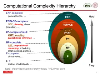
Complexity for Deep Learning Models of complexity Computational (algorithmic) complexity Kolmogorov complexity Information complexity System complexity Physical complexity (space) Others?

Impact The efficiency of algorithms/methods The inherent "difficulty" of problems of practical and/or theoretical importance A major discovery in the science was that computational problems can vary tremendously in the effort required to solve them precisely. The technical term for a hard problem is "NP-complete" which essentially means: "abandon all hope of finding an efficient algorithm for the exact (and sometimes approximate) solution of this problem". Liars vs damn liars

Optimality A solution to a problem is sometimes stated as optimal Optimal in what sense? Empirically? Theoretically? (the only real definition) Cause we thought it to be so? - weak Different from best If not optimal , then best

Which algorithm to use? An algorithm for solving a problem is not unique. Which one should we use? Based on cost Number of inputs Number of outputs Number of units Time (time vs space) Likely to succeed etc Most solutions often based on similar problems

Good source of algorithms http://www.nist.gov/dads/

Scenarios I ve got two algorithms that accomplish the same task Which is better? I want to store some data How do my storage needs scale as more data is stored Given an algorithm, can I determine how long it will take to run? Input is unknown Don t want to trace all possible paths of execution For different input, can I determine how an algorithm s runtime changes?

Measuring the Growth of Work or Hardness of a Problem While it is possible to measure the work done by an algorithm for a given set of input, we need a way to: Measure the rate of growth of an algorithm based upon the size of the input (or output) Compare algorithms to determine which is better for the situation Compare and analyze for large problems Examples of large problems?

Time vs. Space Very often, we can trade space for time: For example: maintain a collection of students with ID information. Use an array of a billion elements and have immediate access (better time) Use an array of number of students and have to search (better space)

Introducing Big O Notation Will allow us to evaluate algorithms. Has precise mathematical definition Used in a sense to put algorithms into families Worst case scenario What does this mean? Other types of cases?

Why Use Big-O Notation Used when we only know the asymptotic upper bound. What does asymptotic mean? What does upper bound mean? If you are not guaranteed certain input, then it is a valid upper bound that even the worst-case input will be below. Why worst-case? May often be determined by inspection of an algorithm.

Size of Input (measure of work) In analyzing rate of growth based upon size of input, we ll use a variable Why? For each factor in the size, use a new variable n is most common Examples: A linked list of n elements A 2D array of n x m elements A Binary Search Tree of p elements

Formal Definition of Big-O For a given function g(n), O(g(n)) is defined to be the set of functions O(g(n)) = {f(n) : there exist positive constants c and n0 such that 0 f(n) cg(n) for all n n0}

Visual O( ) Meaning cg(n) Upper Bound f(n) f(n) = O(g(n)) Work done Our Algorithm n0 Size of input

Simplifying O( ) Answers We say Big O complexity of 3n2 + 2 = O(n2) drop constants! because we can show that there is a n0 and a c such that: 0 3n2 + 2 cn2 for n n0 i.e. c = 4 and n0 = 2 yields: 0 3n2 + 2 4n2 for n 2 What does this mean?

Simplifying O( ) Answers We say Big O complexity of 3n2 + 2n = O(n2) + O(n) = O(n2) drop smaller!

Correct but Meaningless You could say 3n2 + 2 = O(n6) or 3n2 + 2 = O(n7) But this is like answering: What s the world record for the mile? Less than 3 days. How long does it take to drive to Chicago? Less than 11 years.

Comparing Algorithms Now that we know the formal definition of O( ) notation (and what it means) If we can determine the O( ) of algorithms This establishes the worst they perform. Thus now we can compare them and see which has the better performance.

Comparing Factors N2 N Work done log N 1 Size of input

Correctly Interpreting O( ) O(1) or Order One Does not mean that it takes only one operation Does mean that the work doesn t change as n changes Is notation for constant work O(n) or Order n Does not mean that it takes n operations Does mean that the work changes in a way that is proportional to n Is a notation for work grows at a linear rate

Complex/Combined Factors Algorithms typically consist of a sequence of logical steps/sections We need a way to analyze these more complex algorithms It s easy analyze the sections and then combine them!

Example: Insert in a Sorted Linked List Insert an element into an ordered list Find the right location Do the steps to create the node and add it to the list 17 38 head // 142 Step 1: find the location = O(N) Inserting 75

Example: Insert in a Sorted Linked List Insert an element into an ordered list Find the right location Do the steps to create the node and add it to the list 17 38 head // 142 75 Step 2: Do the node insertion = O(1)

Combine the Analysis Find the right location = O(n) Insert Node = O(1) O(n) Sequential, so add: O(n) + O(1) = O(n + 1) = Only keep dominant factor

Example: Search a 2D Array Search an unsorted 2D array (row, then column) Traverse all rows For each row, examine all the cells (changing columns) 1 2 3 4 5 1 2 3 4 5 6 7 8 9 10 O(N) Row Column

Example: Search a 2D Array Search an unsorted 2D array (row, then column) Traverse all rows For each row, examine all the cells (changing columns) 1 2 3 4 5 1 2 3 4 5 6 7 8 9 10 Row Column O(M)

Combine the Analysis Traverse rows = O(N) Examine all cells in row = O(M) Embedded, so multiply: O(N) x O(M) = O(N*M)

Sequential Steps If steps appear sequentially (one after another), then add their respective O(). N loop . . . endloop loop . . . endloop O(N + M) M

Embedded Steps If steps appear embedded (one inside another), then multiply their respective O(). loop loop . . . endloop endloop O(N*M) M N

Correctly Determining O( ) Can have multiple factors: O(NM) O(logP + N2) But keep only the dominant factors: O(N + NlogN) O(N*M + P) O(V2 + VlogV) Drop constants: O(2N + 3N2) O(NlogN) O(N*M) O(V2) What about O(NM) & O(N2)? O(N2) O(N + N2)

Summary We use O() notation to discuss the rate at which the work of an algorithm grows with respect to the size of the input. O() is an upper bound, so only keep dominant terms and drop constants

Best vs worse vs average Best case is the best we can do Worst case is the worst we can do Average case is the average cost Which is most important? Which is the easiest to determine?

Poly-time vs expo-time Such algorithms with running times of orders O(log n), O(n ), O(n log n), O(n2), O(n3) etc. Are called polynomial-time algorithms. On the other hand, algorithms with complexities which cannot be bounded by polynomial functions are called exponential-time algorithms. These include "exploding- growth" orders which do not contain exponential factors, like n!.

The Traveling Salesman Problem The traveling salesman problem is one of the classical problems in computer science. A traveling salesman wants to visit a number of cities and then return to his starting point. Of course he wants to save time and energy, so he wants to determine the shortest path for his trip. We can represent the cities and the distances between them by a weighted, complete, undirected graph. The problem then is to find the circuit of minimum total weight that visits each vertex exactly once.

The Traveling Salesman Problem Example: What path would the traveling salesman take to visit the following cities? Toronto 650 550 700 Boston 700 Chicago 200 600 New York Solution: The shortest path is Boston, New York, Chicago, Toronto, Boston (2,000 miles).

Costs as computers get faster

The Towers of Hanoi A B C Goal: Move stack of rings to another peg Rule 1: May move only 1 ring at a time Rule 2: May never have larger ring on top of smaller ring

Towers of Hanoi: Solution Original State Move 1 Move 2 Move 3 Move 5 Move 4 Move 6 Move 7

Towers of Hanoi - Complexity For 3 rings we have 7 operations. In general, the cost is 2N 1 = O(2N) Each time we increment N, we double the amount of work. This grows incredibly fast!

Towers of Hanoi (2N) Runtime For N = 64 2N = 264 = 18,450,000,000,000,000,000 If we had a computer that could execute a billion instructions per second It would take 584 years to complete But it could get worse

Where Does this Leave Us? Clearly algorithms have varying runtimes or storage costs. We d like a way to categorize them: Reasonable, so it may be useful Unreasonable, so why bother running

Performance Categories of Algorithms Sub-linear O(Log N) Linear O(N) Nearly linear O(N Log N) Quadratic O(N2) Polynomial Exponential O(2N) O(N!) O(NN)

Reasonable vs. Unreasonable Reasonable algorithms have polynomial factors O (Log N) O (N) O (NK) where K is a constant Unreasonable algorithms have exponential factors O (2N) O (N!) O (NN)

Reasonable vs. Unreasonable Reasonable algorithms May be usable depending upon the input size Unreasonable algorithms Are impractical and useful to theorists Demonstrate need for approximate solutions Remember we re dealing with large N (input size)

Two Categories of Algorithms Unreasonable 1035 1030 1025 1020 1015 trillion billion million 1000 100 10 NN 2N Runtime N5 Reasonable N Don t Care! 2 4 8 16 32 64 128 256 512 1024 Size of Input (N)