Computational Learning Theory: Insights into PAC Learning Theorem and VC Dimension

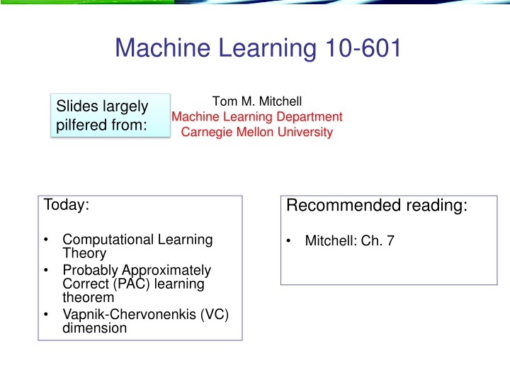
Machine Learning 10-601 Tom M. Mitchell Machine Learning Department Carnegie Mellon University Slides largely pilfered from: Recommended reading: Today: Computational Learning Theory Probably Approximately Correct (PAC) learning theorem Vapnik-Chervonenkis (VC) dimension Mitchell: Ch. 7

Computational Learning Theory What general laws constrain learning? What can we derive by analysis? * See annual Conference on Computational Learning Theory

Computational Learning Theory What general laws constrain learning? What can we derive by analysis? An successful analysis for computation: the time complexity of a program. Predict running time as a function of input size (actually we upper bound it) Can we predict error rate as a function of sample size? (or upper bound it?) sample complexity What sort of assumptions do we need to make to do this? * See annual Conference on Computational Learning Theory

Sample Complexity How many training examples suffice to learn target concept? (eg, a linear classifier, or a decision tree)? What exactly do we mean by this? Usually: There is a space of possible hypotheses H (e.g., binary decision trees) In each learning task, there is a target concept c (usually c is in H). There is some defined protocol where the learner gets information.

Sample Complexity How many training examples suffice to learn target concept? 1. If learner proposes instances as queries to teacher? - learner proposes x, teacher provides c(x) 2. If teacher (who knows c) proposes training examples? - teacher proposes sequence {<x1, c(x1)>, <xn, c(xn)> 3. If some random process (e.g., nature) proposes instances, and teacher labels them? - instances x drawn according to P(X), teacher provides label c(x)

A simple setting to analyze Problem setting: Set of instances Set of hypotheses Set of possible target functions Set of m training instances drawn from teacher provides noise-free label Learner outputs any consistent Find c? Question: how big should m be (as a function of H) for the learner to succeed? Find an h that approximates c? But first - how do we define success ?

The true error of h is the probability that it will misclassify an example drawn at random from Usually we can t compute this but we might be able to prove things about it

A simple setting to analyze Problem setting: Set of instances Set of hypotheses Set of possible target functions Set of m training instances drawn from teacher provides noise-free label Learner outputs any consistent Question: how big should m be (as a function of H) to guarantee that What if we happen to get a really bad set of examples? errortrue(h) < ?

A simple setting to analyze Problem setting: Set of instances Set of hypotheses Set of possible target functions Sequence of m training instances drawn from teacher provides noise-free label Learner outputs any consistent Question: how big should m be to ensure that ProbD[ errortrue(h) < ] > 1- This criterion is called probably approximately correct (pac learnability)

Valiants proof

Valiants proof Assume H is finite, and let h* be learner s output Fact: for in [0,1], (1- ) e- Consider a bad h, where errortrue(h) > Prob[ h consistent with x1 < (1- ) e- ] Prob[ h consistent with all of x1 , xm < (1- )m e- m] Prob[ h* is bad ] = Prob[ errortrue(h*) > ] < |H|e- m (union bound) How big does m have to be?

Valiants proof Assume H is finite, and let h* be learner s output How big does m have to be? Let s solve: Prob[ errortrue(h*) > ] < |H|e- m< He-em<d e-em<d H -em < lnd H em > lnH d m >1 =1 lnH +ln1 elnH d e d

Pac-learnability result Problem setting: Set of instances Set of hypotheses Set of possible target functions Set of m training instances drawn from P(X), with noise- free labels If the learner outputs any h from H consistent with the data and m >1 e d lnH +ln1 logarithmic in |H| linear in 1/ then ProbD[ errortrue(h) < ] > 1-

Stopped Tues 10/6

Notation: VSH,D = { h | h consistent with D} E.g., X=< X1, X2, ... Xn > Each h H constrains each Xi to be 1, 0, or don t care In other words, each h is a rule such as: If X2=0 and X5=1 Then Y=1, else Y=0 Q:How do we find a consistent hypothesis? A: Conjoin all constraints that are true off all positive examples

Pac-learnability result Problem setting: Let X = {0,1}n, H=C={conjunctions of features} This is pac-learnable in polynomial time, with a sample complexity of

Comments on pac-learnability This is a worst case theory We assumed the training and test distribution were the same We didn t assume anything about P(X) at all, expect that it doesn t change from train to test The bounds are not very tight empirically you usually don t need as many examples as the bounds suggest We did assume clean training data this can be relaxed

Another pac-learnability result Problem setting: Let X = {0,1}n, H=C=k-CNF = {conjunctions of disjunctions of up to k features} <= k Example: (x1 x7) (x3 x5 x6) ( x1 x2) This is pac-learnable in polynomial time, with a sample complexity of m 1 e nkln3+ln1 d Proof: it s equivalent to learning in a new space X with nk features, each corresponding to a length-k disjunction

Pac-learnability result Problem setting: Let X = {0,1}n, H=C=k-term DNF = {up to k disjunctions of conjunctions of any # of features} (x1 x3 x5 x7) ( x2 x3 x5 x6) Example: The sample complexity is polynomial, but it s NP-hard to find a consistent hypothesis! Proof of sample complexity: for any h, the negation of h is in our last H. (Conjunctions of length-k disjunctions). So H is not larger than k-CNF. In fact - k-term-DNF is a subset of k-CNF

Pac-learnability result Problem setting: Let X = {0,1}n, H=k-CNF, C=k-term-DNF This is pac-learnable in polynomial time, with a sample complexity of m 1 e nkln3+ln1 d I.e. k-term NDF is pac-learnable by k-CNF An increase in sample complexity might be worth suffering if it decreases the time complexity

Pac-learnability result Problem setting: Let X = {0,1}n, H = {boolean functions that can be written down in a subset of Python} Eg: (x[1] and not x[3]) or (x[7]==x[9]) Hn = { h in H | h can be written in n bits or less} Learning algorithm: return the simplest consistent hypothesis h. I.e.: if h in Hn, then for all j<n, no h in Hj is consistent This is pac-learnable (not in polytime), with a sample complexity of m 1 e nln2+ln1 d

Pac-learnability result (Occams razor) Problem setting: Let X = {0,1}n, H=C=F = {boolean functions that can be written down in a subset of Python} Fn = { f in F | f can be written in n bits or less} Learning algorithm: return the simplest consistent hypothesis h. This is pac-learnable (not in polytime), with a sample complexity of m 1 e d nln2+ln1 H4 H3 H2 H1

VC DIMENSION AND INFINITE HYPOTHESIS SPACES

Pac-learnability result: what if H is not finite? Problem setting: Set of instances Set of hypotheses Set of possible target functions Set of m training instances drawn from P(X), with noise- free labels If the learner outputs any h from H consistent with the data and m >1 e d lnH +ln1 Can I find some property like ln|H| for perceptrons, neural nets, ? then ProbD[ errortrue(h) < ] > 1-

a labeling of each member of S as positive or negative

VC(H)>=3

Pac-learnability result: what if H is not finite? Problem setting: Set of instances Set of hypotheses/target functions H=C where VC(H)=d Set of m training instances drawn from P(X), with noise- free labels If the learner outputs any h from H consistent with the data and then ProbD[ errortrue(h) < ] > 1- Compare:

VC dimension: An example Consider H = { rectangles in 2-D space } and X = {x1,x2,x3} below. Is this set shattered? x3 x1 x2

VC dimension: An example Consider H = { rectangles in 2-D space } Is this set shattered? x3 x1 x2

VC dimension: An example Consider H = { rectangles in 2-D space } Is this set shattered? x3 x1 x2 Yes: every dichotomy can be expressed by some rectangle in H

VC dimension: An example Consider H = { rectangles in 2-D space } and X = {x1,x2,x3,4} below. Is this set shattered? x3 x1 x4 x2 No: I can t include {x1,x2,x3} in a rectangle without including x4.

VC dimension: An example Consider H = { rectangles in 2-D space } and X = {x1,x2,x3,4} below. Is this set shattered? x3 x1 x4 x2

VC dimension: An example Consider H = { rectangles in 2-D space } and X = {x1,x2,x3,4} below. Is this set shattered? x3 x1 x4 x2 Yes: every dichotomy can be expressed by some rectangle in H

VC dimension: An example Consider H = { rectangles in 2-D space }. Can you shatter any set of 5? So the VC(H)=4 x3 x1 x5 x4 x2 No: consider x1 = min(horizontal), x2=max(horizontal), x3=min(vertical), x4=max(vertical), and let x5 the last point. If you include x1 x4, you must include x5.

VC dimension: An example Consider H = { rectangles in 3-D space }. What s the VC dimension? x3 x1 x5 x4 x2

Pac-learnability result: what if H is not finite? Problem setting: Set of instances Set of hypotheses/target functions H=C where VC(H)=d Set of m training instances drawn from P(X), with noise- free labels If the learner outputs any h from H consistent with the data and m O1 e dlog1 e+log1 d then ProbD[ errortrue(h) < ] > 1- compare: m O1 log H +log1 e d

Intuition: why large VC dimension hurts Suppose you have labels of all but one of the instances in X, you know the labels are consistent with something in H, and X is shattered by H. No: you need at least VC(H) examples before you can start learning Can you guess label of the final element of X?

Intuition: why small VC dimension helps We don t need to worry about h s that classify the data exactly the same. x12 How many rectangles are there that are different on the sample S, if |S|=m? x1 x14 x13 x3 x15 x4 Claim: choose(m,4). Every 4 positive points defines a distinct-on-the-data h. x3 x16 x9 x8 x11 x5 This can be generalized: if VC(H)=d, then the number of distinct-on-the-data hypotheses grows as O(md). x7 x6 x10

Tightness of Bounds on Sample Complexity How many examples m suffice to assure that any hypothesis that fits the training data perfectly is probably (1- ) approximately ( ) correct? How tight is this bound? Lower bound on sample complexity (Ehrenfeucht et al., 1989): Consider any class C of concepts such that VC(C) > 1, any learner L, any 0 < < 1/8, and any 0 < < 0.01. Then there exists a distribution and a target concept in C, such that if L observes fewer examples than Then with probability at least , L outputs a hypothesis with

AGNOSTIC LEARNING AND NOISE

Here is the difference between the training error and true error of the output hypothesis (the one with lowest training error)

Additive Hoeffding Bounds Agnostic Learning Given m independent flips of a coin with true Pr(heads) = we can bound the error in the maximum likelihood estimate Relevance to agnostic learning: for any single hypothesis h But we must consider all hypotheses in H (union bound again!) So, with probability at least (1- ) every h satisfies

Agnostic Learning: VC Bounds [Sch lkopf and Smola, 2002] With probability at least (1- ) every h H satisfies

Structural Risk Minimization [Vapnik] Which hypothesis space should we choose? Bias / variance tradeoff H4 H3 H2 H1 SRM: choose H to minimize bound on expected true error! * this is a very loose bound...

MORE VC DIMENSION EXAMPLES

VC dimension: examples Consider X = <, want to learn c:X {0,1} What is VC dimension of Open intervals: x Closed intervals:

VC dimension: examples Consider X = <, want to learn c:X {0,1} What is VC dimension of Open intervals: x VC(H1)=1 VC(H2)=2 Closed intervals: VC(H3)=2 VC(H4)=3

VC dimension: examples What is VC dimension of lines in a plane? H2 = { ((w0 + w1x1 + w2x2)>0 y=1) }

VC dimension: examples What is VC dimension of H2 = { ((w0 + w1x1 + w2x2)>0 y=1) } VC(H2)=3 For Hn = linear separating hyperplanes in n dimensions, VC(Hn)=n+1