Computational Methods for Ordinary Differential Equations in Engineering
Explore numerical methods like Euler Forward, Adams-Bashforth, and Runge-Kutta for solving Initial Value Problems and System of ODEs. Understand concepts of higher-order IVPs and Boundary Value Problems. Gain insights into the application of multi-step and implicit methods for accurate solutions.

Download Presentation

Please find below an Image/Link to download the presentation.
The content on the website is provided AS IS for your information and personal use only. It may not be sold, licensed, or shared on other websites without obtaining consent from the author. If you encounter any issues during the download, it is possible that the publisher has removed the file from their server.
You are allowed to download the files provided on this website for personal or commercial use, subject to the condition that they are used lawfully. All files are the property of their respective owners.
The content on the website is provided AS IS for your information and personal use only. It may not be sold, licensed, or shared on other websites without obtaining consent from the author.
E N D
Presentation Transcript
Ordinary Differential Equation The methods for Initial Value Problems (IVPs): Multi-step Methods Explicit: Euler Forward, Adams-Bashforth Implicit: Euler Backward, Trapezoidal and Adams-Moulton Backward Difference Formulae (BDF) Runge-Kutta Methods Applications, Startup, Combination Methods (Predictor- Corrector) Consistency, Stability, Convergence Application to System of ODEs Boundary Value Problems (BVPs) Shooting Method Direct Methods
ESO 208A: Computational Methods in Engineering Ordinary Differential Equation: System of IVPs and Higher Order IVPs Abhas Singh Department of Civil Engineering IIT Kanpur Acknowledgements: Profs. Saumyen Guha and Shivam Tripathi (CE)
System of IVPs A general non-linear system of IVPs: ??1 ??= ?1(?1,?2 ??,? ??2 ?? ??? ?? ?1= ?1,?2= ?2, ??= ?? at ? = 0 If we write them in the vector form: ?? ??= ? ?,? If the function fi s are linear: ?? ??= ?? + ? Initial Condition: y = a at t = 0 = ?2(?1,?2 ??,? = ??(?1,?2 ??,?
Higher Order IVP A general mth order IVP: ??= ? ?? 1,?? 2, ? ,?;? ? = ?0, ? = ?1, ? = ?2, ?? 1= ?? 1 at ? = 0 Define a set of variables ?1,?2,?3, ?? as, ?1= ?, ?2= ? , ?3= ? , ??= ?? 1 The mth order IVP can be written as a system of IVPs in terms of the new variables as: ?1 ?2 ?3 ?? 1 = ?? ?? ?1 = ?2 = ?3 = ?4 = ? ?1,?2,?3, ??;? 0= ?0, ?2 0= ?1, ?3 0= ?2, ?? 0= ?? 1 at ? = 0
Higher Order IVP: Example Consider the 2nd order IVP: ?2? ?? + ? =1 ? ? 1, ? 1 = 0 ? 1 = 0 Define: ?1= ?, ?2= ? The 2nd order IVP can be written as a linear system of IVPs: ?1 =?2 ?3 ?2 ?? ??= ?? + ? ?11 = 0 ?21 = 0 = ?2 0 1 1 ? 0 1 ?3 = ? ?1 ?2+1 ?1 ?2+ ?1 1 ?2 ?2
Numerical Methods for System of IVPs All methods developed for the IVPs are also applicable for the system of IVPs Substitute the variables y and f for the vectors of variables y and f Example: Euler Forward ?? ??= ? ?,? ??+?= ??+ ?? ? ?? ? ?? ?,?2 ?,?2 ?,?2 0 ?+1 ? ?,?? ?,?? ?1(?1 ?2(?1 ?1 ?2 ?1 ?2 ?? ?1 ?2 ?? ? ?+1 0 ; ?0= = + ?+1 ? ?? ?,?? ? 0 ??(?1 ??
Numerical Methods for System of IVPs Example: Euler Backward (Linear f) ?? ??= ?? + ? ??+?= ??+ ??+?= ??+ ??+???+?+ ??+? ? ??+???+?= ??+ ??+? 0 ?1 ?2 ?? 0 ?0= 0 A and b are functions of t only. Therefore, they are known at all time steps.
Numerical Methods for System of IVPs Example: Euler Backward (Non-linear f) ?? ??= ? ?,? ??+?= ??+ ??+? ?+1 ?? ?+1 ?? ?+1 ?? ?+1,?2 ?+1,?2 ?+1 ? ?+1,??+1 ?+1,??+1 ?1(?1 ?2(?1 ?1 ?2 ?1 ?2 ?? ? ?+1 = + ; ?+1 ? ?+1,?2 ?+1,??+1 ??(?1 ?? 0 ?1 ?2 ?? 0 ?0= 0
Numerical Methods for System of IVPs Example: Euler Backward (Non-linear f) ??+?= ??+ ??+? ??+? ??+? ??= ? ?+1 ?? ?+1 ?? ?+1 ?? ?+1,?2 ?+1,?2 ?+1 ? ?+1,??+1 ?+1,??+1 ?1(?1 ?2(?1 ?1 ?2 ?1 ?2 ?? ? ?+1 = 0 ?+1 ? ?+1,?2 ?+1,??+1 ??(?1 ?? Recall Newton-Raphson method for the system of non-linear equations: ? ?? ?(?+1 ?(? = ? ?(? ? ?? ??+? ?+? ?+? ?? ?+?= ?? ?+?+ ?? ?+?+ ?? k is the iteration index for the Newton-Raphson
Numerical Methods for System of IVPs ??1 ??1 ??2 ??1 ??? ??1 ??1 ??2 ??2 ??2 ??? ??2 ??1 ??? ??2 ??? ??? ??? ? = Note for Application: One may not update the Jacobian at every iteration of the Newton-Raphson Calculate it after every 4-5 iterations or when iteration slows down.
Example application: Higher Order IVP ? + ??? + ? 1 ? 2 ? 0 = 0; ? 0 = 0; ? 0 = 5.0 = 0 ? 0,1 Formulate the System of IVPs: Define: ? = ?, ? = ? and ? = ? ? = ? ? = ? ? = ??? ? 1 ?2 Initial Conditions: ? 0 = 0, ? 0 = 0, ? 0 = 5.0 This is equivalent to: ? ? ? ? ? ?? ??= ? ?,? ? = ; ? ?,? = ??? ? 1 ?2
Example application: Higher Order IVP ? + ??? + ? 1 ? 2 ? 0 = 0; ? 0 = 0; ? 0 = 10.0; ? = 1.0; ? = 1.0 = 0 ? 0,1 Define: ? = ?, ? = ? and ? = ? ? ? ? ? ? ?? ??= ? ?,? ? = ; ? ?,? = ??? ? 1 ?2 Initial Conditions: ? 0 = 0, ? 0 = 0, ? 0 = 10.0 Euler Forward: ??+?= ??+ ?? ?? ?? ??+ ?? ??+ ?? ??+1 ??+1 ??+1 ?? ?? ?? = + = 2 2 ????? ? 1 ?? ?? ????? ? 1 ??
Example application: Higher Order IVP ? + ??? + ? 1 ? 2 ? 0 = 0; ? 0 = 0; ? 0 = 10.0; ? = 1.0; ? = 1.0 = 0 ? 0,1 Define: ? = ?, ? = ? and ? = ? ? ? ? ? ? ?? ??= ? ?,? ? = ; ? ?,? = ??? ? 1 ?2 Initial Conditions: ? 0 = 0, ? 0 = 0, ? 0 = 10.0 Runge-Kutta 4th Order: 1 6?0+1 3?1+ ?2 +1 ??+1= ??+ 6?3
Example application: Higher Order IVP ? ? ? ? ? ?? ??= ? ?,? ? = ; ? ?,? = ??? ? 1 ?2 Initial Conditions: ? 0 = 0, ? 0 = 0, ? 0 = 10.0 Runge-Kutta 4th Order: ?? ?? ??= ? ??,?? = 2 ????? ? 1 ?? ??= ? ??+1 2 ??,??+1 2 ??+ 2?? ?? ?? ?? ?? ?? ??1 ??1 ??1 ??+1 + ??+ 2 ??= = = 2?? 2 2 ????? ? 1 ?? ?? 2????? 2 2? 1 ?? ??1 ??1 ??= 2 ???1??1 ? 1 ??1
Example application: Higher Order IVP ? ? ? ? ? ?? ??= ? ?,? ? = ; ? ?,? = ??? ? 1 ?2 Initial Conditions: ? 0 = 0, ? 0 = 0, ? 0 = 10.0 Runge-Kutta 4th Order: ??= ? ??+1 2 ??,??+1 2 ??+ 2??1 ??1 ??1 ?? ?? ?? ??2 ??2 ??2 ??+1 + ??+ 2 ??= = = 2??1 2 2 ???1??1 ? 1 ??1 ?? 2???1??1 2 2? 1 ??1 ??2 ??2 ??= 2 ???2??2 ? 1 ??2
Example application: Higher Order IVP ? ? ? ? ? ?? ??= ? ?,? ? = ; ? ?,? = ??? ? 1 ?2 Initial Conditions: ? 0 = 0, ? 0 = 0, ? 0 = 10.0 Runge-Kutta 4th Order: ??= ? ??+ ??,??+ ??2 ??2 ??+ ??2 ??+ ??2 ?? ?? ?? ??+ ??= + = 2 2 ???2??2 ? 1 ??2 ?? ???2??2 ? 1 ??2 ??3 ??3 ??3 = ??3 ??3 ??= 2 ???3??3 ? 1 ??3 1 6?0+1 3?1+ ?2 +1 ??+1= ??+ 6?3
Example application: Higher Order IVP ? ? ? ? ? ?? ??= ? ?,? ? = ; ? ?,? = ??? ? 1 ?2 Initial Conditions: ? 0 = 0, ? 0 = 0, ? 0 = 10.0 Runge-Kutta 4th Order: 1 6?0+1 3?1+ ?2 +1 ??+1= ??+ 6?3 ??+1 ??1 ??1 ?? ?? ?? ?? ?? + + = 6 3 2 2 ???1??1 ? 1 ??1 ????? ? 1 ?? ??2 ??2 ??3 ??3 + + 3 6 2 2 ???2??2 ? 1 ??2 ???3??3 ? 1 ??3
Example application: Higher Order IVP ? + ??? + ? 1 ? 2 ? 0 = 0; ? 0 = 0; ? 0 = 10.0; ? = 1.0; ? = 1.0 = 0 ? 0,1 Define: ? = ?, ? = ? and ? = ? ? ? ? ? ? ?? ??= ? ?,? ? = ; ? ?,? = ??? ? 1 ?2 Initial Conditions: ? 0 = 0, ? 0 = 0, ? 0 = 10.0 Euler Backward: ??+?= ??+ ??+? ??+? ??+? ??= ? ?+? ?+? ?? ?+?= ?? ?+?+ ?? ?+?+ ?? ? ?? ??+?
Example application: Higher Order IVP ? ? ? ? ? ?? ??= ? ?,? ? = ; ? ?,? = ??? ? 1 ?2 Initial Conditions: ? 0 = 0, ? 0 = 0, ? 0 = 10.0 Euler Backward: ? ?? ?+? ?+? ?? ?+?= ?? ?+?+ ?? ?+?+ ?? ??+? 0 0 1 0 0 1 ? = ?? 2?? ?? ?+1 ?? ?+1 ?? ?+1 ?? ?+1 ??+1 ??+1 ??+1 1 0 1 0 ?+1 ?+1 ?+1 ?+1 ? ?? 2? ?? 1 + ? ?? ?+1 ?+1+ ?? ?+1+ ?? ?+1 ? 1 ?? ?+1+ ?? ?+1+ ?? ?? ?? ?+1?? = ?+12 ?+1 ? ?? + ?? ??
Example application: Higher Order IVP Euler Backward: Stop Newton-Raphson iteration and take the next time step when, ?+? ?? ?? ?+? ??+? ? ?+?
Stability of the System of IVPs Model Equation: ?? ??= ?? Example: Euler Forward ??+?= ? + ? ?? Define: ??+? ?? For Stability: ??+? ?? If the maximum eigenvalue of A is max: ??+? ?? ? + ? ? = ? = ? + ? < ? ? ? + ? 1 2 1 + ?max 1 ?max
Stability of the System of IVPs In higher order IVP or in a system of IVP, the solutions are characterized by the eigenvalues. One or two equation in the system typically have high eigenvalues close to max and the rest of the equations may have eigenvalues of much lower magnitudes! The time step is restricted by max. Stiff system: large value of ( max/ min); typically > 100 As the time progresses, larger time step can be used for the problem but is limited by the stability criteria! This is the utility of the BDFs: They are stable for all real and negative R up to 6th order Region of stability for imaginary I increases as one increases the time step (increasing Rh)!
Example: Stiff System ? = 50? ? = 50? 0.1? + ? ? 0 = 1, In higher order IVP or in a system of IVP, the solutions are characterized by the eigenvalues: ? 0 = 0, ? 0, Eigenvalues are -50 and -0.1 ???? ???? = 500, therefore, it s a Stiff System Analytical Solution: ? = ? 50? and ? = 1.002? 50?+ 98.998? 0.1?+ 10? 100 Essentially, two time scales defined by two eigenvalues! We need a fine grid or time step to resolve the fast decaying solution and large time step can be used to resolve the slow decay/growth Methods like Euler Forward or any such method with limited allowable time step size will not allow this!
Stability: BDF Methods Example For all the BDFs: Stability Region is outside the enclosed region! For real , all the BDFs are unconditionally stable! One can use any h without having to worry about the stability! Useful for stiff equations!
Stability of the System of IVPs In order to resolve the fast decaying part, choose initial time step of h = 1/ max and use first order BDF or BDF1. Increase h and switch to BDF2 after a few time step Increase h and switch to BDF3 Proceed like this all the way to BDF6 Remember, you do not need to worry about stability unless it is purely imaginary ! Two examples for the same problem! ? = 50? ? = 50? 0.1? + ? ? 0 = 1, ? 0 = 0, ? 0,
Method h t 0 u v 1.00E+00 6.67E-01 4.44E-01 2.96E-01 1.98E-01 1.32E-01 -5.92E-02 -4.60E-02 -1.56E-02 5.49E-02 2.46E-02 -1.99E-03 -3.61E-03 -2.97E-02 -5.90E-03 4.52E-03 -2.44E-04 -1.24E-03 1.85E-03 3.26E-03 -3.90E-04 -4.31E-04 3.63E-04 -4.63E-05 -4.08E-03 -8.42E-04 0.0000 -0.3329 -0.5544 -0.7015 -0.7991 -0.8636 -1.0460 -1.0217 -0.9776 -0.8725 -0.8588 -0.8319 -0.7706 -0.6428 -0.4285 -0.1917 0.0648 0.3596 1.0548 1.8780 2.8208 3.8870 5.0691 6.3605 9.2541 12.5474 BDF1 0.01 0.01 0.01 0.01 0.01 0.05 0.05 0.05 0.1 0.1 0.1 0.1 0.2 0.2 0.2 0.2 0.2 0.4 0.4 0.4 0.4 0.4 0.4 0.8 0.8 0.01 0.02 0.03 0.04 0.05 0.1 0.15 0.2 0.3 0.4 0.5 0.6 0.8 1 1.2 1.4 1.6 2 2.4 2.8 3.2 3.6 4 4.8 5.6 BDF2 BDF3 BDF4 BDF5 BDF6
Method h t 0 u v 1.00E+00 5.00E-01 2.50E-01 0.00E+00 -3.57E-02 -2.04E-02 4.66E-02 2.92E-02 1.88E-03 -3.89E-03 -3.77E-02 -9.44E-03 6.24E-03 3.92E-04 -2.01E-03 -1.98E-04 4.53E-03 8.73E-05 -1.05E-03 5.08E-04 1.29E-04 -4.81E-03 -1.45E-03 0.0000 -0.4986 -0.7463 -0.9903 -1.0181 -0.9932 -0.9024 -0.8900 -0.8815 -0.8451 -0.7767 -0.6222 -0.4570 -0.2904 -0.0977 0.3607 0.9086 1.5310 2.2378 3.0257 3.8877 5.8257 8.0484 BDF1 0.02 0.02 0.04 0.04 0.04 0.08 0.08 0.08 0.08 0.16 0.16 0.16 0.16 0.16 0.32 0.32 0.32 0.32 0.32 0.32 0.64 0.64 0.02 0.04 0.08 0.12 0.16 0.24 0.32 0.4 0.48 0.64 0.8 0.96 1.12 1.28 1.6 1.92 2.24 2.56 2.88 3.2 3.84 4.48 BDF2 BDF3 BDF4 BDF5 BDF6
ESO 208A: Computational Methods in Engineering Partial Differential Equations: Introduction, Parabolic Equation Department of Civil Engineering IIT Kanpur
Introduction A general 2nd Order PDE: ????+ 2????+ ????+ ???+ ???+ ? ?,?,? = 0 ?2 ?? = 0: Parabolic PDE, e.g., Diffusion and Advection-Diffusion Equation ?2 ?? < 0: Elliptic PDE, e.g., Laplace Equation ?2 ?? > 0: Hyperbolic PDE, e.g., Wave equation We will learn a few Finite Difference methods for most common PDEs in Engineering Problems!
Parabolic PDE: semi-discretization ?? ??= ??2? ? 0,? = ?0; ? ?,? = ??; ? ?,0 = ? ? ??= ??2? ?? ??+ ??? ??2 ??2 ??? ?? ??? ?? ??+1 2??+ ?? 1 ??2 ??+1 ?? 1 2?? = ?? ??+1 2??+ ?? 1 ??2 = ?? + ??
Parabolic PDE: semi-discretization ?? ??= ??2? ? 0,? = ?0; ? ?,? = ??; ? ?,0 = ? ? ; ? = 4 ??? ?? ??+1 2??+ ?? 1 ??2 ??2 = ?? ??1 ?? ??2 ?? ??3 ?? 2?1 ??2 ?2 ??2 ?1 ??2 2?2 ??2 ?3 ??2 ?0?1 ??2 0 ???3 ??2 0 ?1 ?2 ?3 ?2 ??2 2?3 ??2 = + 0
Parabolic PDE: semi-discretization ??= ??2? ?? ??+ ??? ? 0,? = ?0; ? ?,? = ??; ? ?,0 = ? ? ??? ?? ??+1 ?? 1 2?? ??+1 2??+ ?? 1 ??2 ??2 = ?? + ?? ??1 ?? ??2 ?? ??3 ?? 2?1 ??2 ?2 2??+ ?1 2??+ 2?2 ??2 ?3 2??+ ?1 ??2 ?1?0 2??+?0?1 0 ?3?? 0 ?1 ?2 ?3 ??2 ?2 ??2 ?2 2??+ 2?3 ??2 ?2 ??2 = + 2??+???3 ?3 ??2 ??2 0
Parabolic PDE: semi-discretization ?? ??= ??2? ? 0,? = ?0; ? ?,? = ??; ? ?,0 = ? ? ??= ??2? ?? ??+ ??? ??2 ??2 ? ?1 ? ?2 ? ?3 ?1 ?2 ?3 d ? dt= ? ? + ? ? = ? 0 =
Parabolic PDE: semi-discretization ? ?1 ? ?2 ? ?3 ?1 ?2 ?3 d ? dt= ? ? + ? ? = ? 0 = ??+1= ??+ ?? ? ?? ??+ ??+ 1 ? ??+1 ??+1+ ??+1 = 0: Euler Backward; = 1: Euler Forward = 1/2: Trapezoidal ? ?? 1 ? ??+1 ??+1 = ? + ????? ??+ ?? 1 ? ??+1+ ???