Confidence Intervals and Meta-Analysis in Resolving Research Replication Crisis
Research replication crisis is a major concern in academia. Professor Will G. Hopkins discusses the significance of confidence intervals and meta-analysis in addressing this issue, referencing John Ioannidis' work on false published research findings.

Download Presentation

Please find below an Image/Link to download the presentation.
The content on the website is provided AS IS for your information and personal use only. It may not be sold, licensed, or shared on other websites without obtaining consent from the author.If you encounter any issues during the download, it is possible that the publisher has removed the file from their server.
You are allowed to download the files provided on this website for personal or commercial use, subject to the condition that they are used lawfully. All files are the property of their respective owners.
The content on the website is provided AS IS for your information and personal use only. It may not be sold, licensed, or shared on other websites without obtaining consent from the author.
E N D
Presentation Transcript
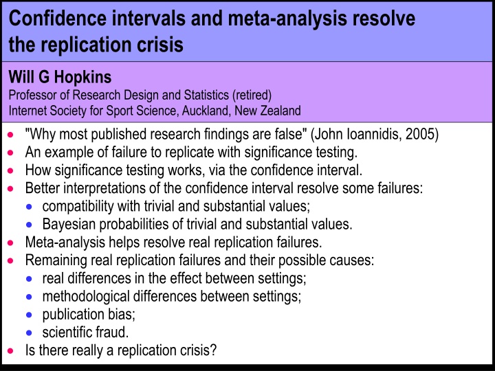
Confidence intervals and meta-analysis resolve the replication crisis Will G Hopkins Professor of Research Design and Statistics (retired) Internet Society for Sport Science, Auckland, New Zealand "Why most published research findings are false" (John Ioannidis, 2005) An example of failure to replicate with significance testing. How significance testing works, via the confidence interval. Better interpretations of the confidence interval resolve some failures: compatibility with trivial and substantial values; Bayesian probabilities of trivial and substantial values. Meta-analysis helps resolve real replication failures. Remaining real replication failures and their possible causes: real differences in the effect between settings; methodological differences between settings; publication bias; scientific fraud. Is there really a replication crisis?
"Why most published research findings are false" John Ioannidis (2005), PLOS Medicine 19: e1004085 "Simulations show that for most study designs and settings, it is more likely for a research claim to be false than true." The false research claims arise from the "chase for statistical significance". In other words, more than half the published claims that there is a "true relationship" (effect) based on statistical significance are false, because there is actually "no relationship". Presumably researchers are supposed to get statistical non-significance when there is "no relationship". But this approach to making claims about effects is illogical. There is never "no relationship". Effects can be trivial or substantial. With a large-enough sample size, all trivial effects are statistically significant. In any case, Goodman and Greenland immediately criticized the model underlying Ioannidis's simulations. They concluded that Ioannidis's claim is "unfounded." But "we agree that there are more false claims than many would suspect." And the paper "calls attention to the importance of avoiding all forms of bias". So, do we have occasional replication failures but not actually a crisis?
An example of failure to replicate with significance testing Someone does a controlled trial on the mean effect of a new form of training with a sample size like many researchers use, 10+10. They get a statistically significant positive effect: Sample size = 10+10, p<0.05 Sample size = 100+100, p>0.05 negative harmful trivial positive beneficial Effect on performance They conclude the treatment is effective. They submit the study for publication, and it's accepted. But they didn't do a power analysis to determine the required sample size. The required sample size gives an 80% chance of obtaining statistical significance (p<0.05), when the true effect is the smallest important. Someone else does the power analysis and estimates a sample size of 100+100. They repeat the study with that sample size. They get a non-significant effect. They conclude that the treatment is ineffective. They publish. To understand this replication failure, first understand significance testing. Furthermore, it's trivial.
How significance testing works, via the confidence interval Statistical significance = rejection of the nil (null) hypothesis. "Nil", because it's 0 for means, and 1 for effects expressed as ratios. Statistical non-significance = failure to reject the nil hypothesis. It's easy to understand hypothesis testing using confidence intervals. significant, p<0.05 non-significant, p>0.05 negative positive Effect on performance There are various interpretations of the CI. Here's the one the frequentists use The interval represents the expected variability in the value of the effect around an hypothesized true value, if the study were repeated many times. The hypothesized value is zero (nil), for the nil-hypothesis test. Observed values would fall outside the interval only 5% of the time, for a 95% confidence interval. So, if the observed value falls outside the interval, the hypothesis is rejected as being too unlikely, given the data: the effect is significant. Otherwise the nil is not rejected: the effect is non-significant.
But you can instead keep the confidence interval centered on the observed effect: Zero is compatible with the data and model Zero is not compatible with the data and model negative positive Effect on performance Values of the effect within the CI are compatible with the data and analytical model (whatever that means). Values outside the CI are not compatible with the data and analytical model. This is Sander Greenland's interpretation of the CI He therefore prefers compatibility interval. If zero falls outside the CI, zero is not compatible with the data and model. This scenario is obviously the same as rejection of the nil hypothesis The effect is significant. If zero falls inside the CI, zero is compatible with the data and model. This scenario is obviously the same as failure to reject the nil hypothesis The effect is non-significant. So, we still have replication failure. But who cares about the zero?
Better interpretations of the confidence interval resolve some failures Consider instead compatibility with trivial and substantialvalues of the effect. Harmful is not compatible with the data and model Beneficial and trivial are compatible with the data and model harmful trivial beneficial Effect on performance For both effects, harmful is not compatible with the data and model. Equivalently, for both effects, the harmful hypothesis is rejected. Either way, there is no failure to replicate in relation to harmful values. Both effects are compatible with trivial and beneficial values. Equivalently, for both effects, trivial and beneficial hypotheses are not rejected. So, again, there is no failure to replicate. Compatibility is equivalent to hypothesis testing, so it suffers from a similar "dichotomania". But one effect is obviously more compatible with beneficial, and the other is more compatible with trivial. Coming soon: how a Bayesian interpretation deals with this degree of compatibility.
First, more on tests of nil, substantial and trivial (non-substantial) hypotheses When testing any hypothesis, you set a Type-1 error rate or "alpha": the chance of rejecting the hypothesis when the hypothesis is true. Well-defined, up-front error rates are a great property of hypothesis tests. With the nil-hypothesis test, alpha is usually 0.05, or a 5% chance of significance, when the true effect is nil or zero. You acknowledge that 5% of studies will give values large enough (positive or negative) to erroneously reject the nil hypothesis. The nil-hypothesis test is "two-sided", and the corresponding CI is 95%. Probability sampling distribution if effect is nil (zero) 95% CI p = 0.025 nil p = 0.025 hypothesis large values with low probability (p = 0.05) 0 Effect magnitude
Tests of substantial and non-substantial hypotheses are one-sided. Example With a sufficiently large positive observed value of the effect, you reject the non-positive hypothesis. The error rate is highest when the hypothesis is trivial and borderline substantial positive. The error rate is the area of one tail of the normal distribution defining sufficiently large values. An error rate of 5%, or alpha = 0.05, seems reasonable as a default. Hence, an alpha of 0.05 corresponds to a 90% CI. I therefore recommend showing 90% CI for all effects. To justify 90%, state in your Methods section that "Inferiority, superiority and equivalence tests based on coverage of a 90% CI have alphas of 0.05." But for clinically or practically relevant effects, you should effectively use different alphas for rejecting harm and rejecting benefit. There is an easier way to think about it... negative Probability trivial positive 90%CI sampling distribution if effect is borderline trivial-positive non- positive hypothesis p = 0.05 Effect magnitude large values with low probability (p = 0.05)
A Bayesian interpretation of the confidence interval Compatible with the data and model has no practical interpretation. And compatible or notdichotomizes outcomes. So, consider this A 90% confidence interval includes the "true" (huge-sample) value of the effect for 90% of samples. (You can show this easily by simulation.) Therefore, common sense (but not a strict statistician) says that there is a 90% chance that the true effect is contained in the confidence interval. That is, the confidence interval represents uncertainty in the true effect. So, in both these studies, the true effect "could be" beneficial and trivial: beneficial and trivial trivial and beneficial harmful trivial beneficial Effect on performance Most practical statisticians implicitly use this interpretation. Some also refer to precision of estimation of the effect. But strictly, these are Bayesian interpretations of the intervals, which are allowed only if the intervals account for prior uncertainty in the true value. So, imagine that you have prior information or a prior belief, with uncertainty represented by a confidence interval, for one of these effects
This prior This prior represents your belief that the true effect could be anything from large harmful to large beneficial: posterior observed effect prior harmful trivial beneficial Effect on performance The prior is equivalent to the effect in a study with a certain sample size. You combine that sample with your sample. The combination is a weighted mean: the "point" estimates are weighted by the inverse of their standard errors (effectively their CIs) squared. This is Sander Greenland's practical approach to Bayesian analysis. This prior "shrinks" the effect to a slightly smaller posterior value, with a slightly narrower confidence interval. But you are allowed to assert no prior belief about the true effect, which is the equivalent of a prior that is so wide, it does not modify the observed CI. The original CI of your effect is then the CI of the true effect. So, any overlap of CIs from two studies represents values of the true effect that could be the same in those studies. must resolve much of the failure to replicate with significance testing. This realistic interpretation of the CIs
Let's leave aside replication failure and develop the Bayesian interpretation in the next three slides The sampling distribution from which the CI is derived is the probability distribution for the true effect. Example: Hence, you can calculate probabilities that the true effect is substantial positive, substantial negative, and trivial. The probabilities (p) and their complements (1 p) are p values for tests of substantial and non-substantial hypotheses. But it's better to interpret the probabilities qualitatively. I devised a scale that turned out to be like that of the Intergovernmental Panel on Climate Change for communicating probability to the public. A probability can also be interpreted as level of evidence for and/or against the magnitude of the true effect, which is a great way to summarize effects. Probability 90%CI sampling distribution area = 0.53 or 53% area = 0.44 or 44% area = 0.03 or 3% negative trivial Effect magnitude positive
Chances <0.5% 0.5-5% 5-25% 25-75% 75-95% 95-99.5% Probability <0.005 0.005-0.05 0.05-0.25 0.25-0.75 0.75-0.95 0.95-0.995 Qualitative most unlikely very unlikely unlikely possibly likely very likely Evidence against or for strong against very good against good against (weak for) some or modest for (against) good for (weak against) very good for clearly not clear excellent or strong for >99.5% >0.995 most likely These qualitative terms replace di-chotomization with septi-chotomization. Colors of the rainbow (or shades of grey) are better than black and white. You can still use very (un)likely to do hypothesis tests with alphas of 0.05. You can use other probabilities or levels of evidence for decisions about implementing clinically or practically relevant effects. Implement a possibly beneficial effect, provided it is most unlikely harmful. For comparison, p = 0.049 with the right sample size for significance corresponds to a 20% chance of benefit but a ~0.0001% risk of harm. possibly = 25% most unlikely = 0.5%
But don't forget that some assumptions underlie the CI and the probabilities. The sampling distribution is normal. This is never a problem, thanks to the Central Limit Theorem. The measurements are not biased. That is, on average, they are correct. They can be noisy and not biased. The statistical model for the effect is appropriate. No problem for simple comparisons of means. Check residuals vs predicteds for non-uniformity. Include subject characteristics as modifying predictors to adjust for differences in means of groups being compared. Check residuals vs predictors for non-linearity. The smallest important is appropriate. Consider a sensitivity analysis with a realistic range of smallest importants, especially for clinical or practical decisions. The effect applies only to a population similar to your sample. The effect, CI and probabilities apply to that population, not to individuals. Modifying covariates provide effects in subpopulations and partly explain individual differences or individual responses. Some of these assumptions help resolve real failures to replicate Raw, percent or factor? Log transformation? Polynomials? Quantiles? Cubic splines?
Remaining real replication failures and their possible causes Interpretation of confidence intervals as compatibility intervals or as likely ranges of the true value show that this scenario does not represent real failure. But if a repeat of Study 1 with 10x the sample size produced this result, then there is no failure to replicate Study 1, but real failure to replicate Study 2. Possible causes of real replication failure: Real differences in the effect between settings These could arise from differences in mean subject characteristics and/or environmental factors that modify the effect. Some of these can be quantified in a random-effect meta-regression. Methodological differences between settings, including administration of treatments (controls, blinding, timing, dose ); measurement of the dependent variable (assays, test protocols ); processing the dependent variable (standardization, log-transformation ); the statistical model (covariates, repeated measurement ). Some of these can be quantified in a random-effect meta-regression. Study 1 Study 2 Study 1a harmful trivial beneficial Effect on performance
Publication bias Suppose the authors of Study 1 repeated their study with 10x the sample size and got this: The likely scenario is that Study 1 produced an unusually large effect because of large sampling variation with a small sample. The effect in Study 1 was statistically significant, so it got published. Studies of other researchers who got non-significance with similar small studies were either not submitted or not accepted for publication. Hence published effects in small studies are biased towards large values. "P-value hacking" also results in publication bias. Example: a researcher deletes an "outlier" to change p >0.05 to p <0.05. Eliminating significance dichotomania would reduce publication bias. Adequate-precision dichotomania results in trivial publication bias. Peer-reviewed proposals with guaranteed publication is also a solution. Meantime, publication bias can usually be eliminated in a meta-analysis. Major scientific fraud, where a researcher fabricates most or all of the data. Such studies may be detected and eliminated from a meta-analysis. Study 1 Study 1a Study 2 harmful trivial beneficial Effect on performance
Meta-analysis helps resolve real replication failures In a meta-analysis, all effects are expressed in the same units and metric, to allow them to be averaged. When the effects are displayed in a forest plot, failure to replicate then becomes obvious. Example: Study 1 Study 2 Study 3 Study 4 Study 5 Study 6 Study 7 Data are means and confidence intervals Study 8 Study 9 Study 10 Mean harmful trivial beneficial Effect on performance Study 2 is not compatible with Studies 6, 8, 9 and 10. Instead of pairwise analysis for replication failures, random-effect meta-analysis allows estimation of real differences (differences not due simply to sampling variation) between all study-estimates as a standard deviation. This SD represents heterogeneity.
If the heterogeneity SD is clearly substantial, there is replication failure. Part of this SD could be due to differences between studies in subject characteristics, environmental factors, or methods that modify the effect. Some of the modifying effects can be estimated by including them as covariates in a meta-regression meta-analysis. Examples: Gender, by including a "male-ness" covariate, with values ranging from 0 (all females) to 1 (all males). Proportion of athletes, with a similar "athlete-ness" covariate. Blinding, timing and dose of a treatment in controlled trials or crossovers. Effects on performance in different training phases. Account for non-linear effects of covariates, where relevant (e.g., duration). Account for repeated measurement within studies with one or more appropriate additional random effects. Outright methodological mistakes are not uncommon and sometimes spotted during meta-analysis. Delete the study, if you can't correct the mistake. Avoid standardization to combine mean effects: it adds non-biological (artifactual) heterogeneity, due to differences in the standardizing SD. To the extent that covariates account for the differences in the effect between studies, the SD representing heterogeneity will be smaller.
After accounting for known differences in methodologies and characteristics, any remaining heterogeneity could be due to unknown differences between settings. Such heterogeneity is not a problem, provided it's plausible. It may consist of within-study as well as between-study differences. Interpreting its magnitude and uncertainty is crucial. The smallest important is half that for usual effects. It combines with the uncertainty in the meta-analyzed mean effect to become the prediction interval: the uncertainty in the effect in a specific new setting Example: Effect of a new kind of training on team-sport females Study 10 Team-sport females Team-sport males Endurance females Endurance males Study 1 Study 2 Study 3 Study 4 Study 5 Study 6 Study 7 Data are means and confidence intervals Study 8 and other types Study 9 Prediction interval: uncertainty in the mean effect in a new setting of athlete. But some remaining heterogeneity could be due to publication bias and scientific fraud. harmful trivial beneficial Effect on performance
Standard error (SE) Publication bias This was initially investigated with a funnel plot of study-estimate SE vs magnitude. Funnel slope = 1/1.96. Asymmetry in the funnel of studies could be due to missing non- significant effects from studies with small sample sizes. Hence, the trim and fill method to adjust for publication bias: you fabricate missing studies to make the plot symmetrical. Or you can delete studies to make the plot more symmetrical. But the funnel is poorly defined, when heterogeneity smears it out. These methods, and one I devised based on the random-effect solution for heterogeneity, don't work well, especially with substantial publication bias. Better methods have been developed recently. Precision-effect estimate with standard errors (PEESE): in the above plot, studies with larger SEs tend to have larger effects. Hence, you can include SE (better, SE2) as a covariate and adjust the effects to SE=0. SE=0 is equivalent to a study with a huge sample size, therefore unbiased. delete published studies, mostly with p <0.05 missing studies with p >0.05 funnel of the 95% of studies with p >0.05, if true effect = 0 funnel of 95% of all studies, if true effect >0 0 Effect magnitude true effect, if no heterogeneity
Selection models: these estimate and adjust for the lower probability of selection (publication) of non-significant effects. In simulations of meta-analyses with small-sample studies typical of sport and exercise research, publication bias is generally small, and both methods adjust for it reasonably well. Scientific fraud, or "questionable scientific practices" Minor fraud aimed at getting a p value over the line amounts to publication bias and will be adjusted away, at least partly, by PEESE or selection models. There may be subtle but incriminating errors in extensively faked data. Example: in meta-analysis of mean changes, we extract errors of measurement where possible, to allow imputation of standard errors of changes in studies lacking confidence intervals or exact p values. An unrealistically low error of measurement (e.g., ~0.5%, when it should be ~5%) is a red flag, especially if the author does not respond to emails. Variability of counts of injuries could also be unrealistic in faked injury data. Studies with extensively faked data appear to be rare. Where there is reasonable evidence for such a study, it should be excluded from the meta-analysis. Any that are missed will be diluted by the studies with real data. In any case, the authors probably fake them to fit with existing studies.
Conclusion Is there really a replication crisis? I don't think so. Here's why Replication failure is not a question of studies differing in significance and non- significance. Confidence intervals reveal real replication failures. Yes, there aresome, but Meta-analysis quantifies the extent of real replication failures as heterogeneity, which is (or can in principle be) explained by subject and study characteristics. Publication bias, and heterogeneity arising therefrom, can be adjusted away. Fake data are probably not show-stoppers. So, Ioannidis' 2005 publication was over the top, but it "sparked reforms" (Bing AI), hopefully not at the expense of toxic skepticism about science.


")