Converting Logical Query Plans to Physical Query Plans in DBMS
Illustrations and steps involved in the process of converting logical query plans (LQP) to physical query plans (PQP) in database management systems (DBMS), focusing on optimization, algorithm implementation, and handling security issues. The images provide a visual guide to constructing physical query plans from optimized LQPs, including replacing leaf nodes with scan operations and combining scans with other operations.

Download Presentation

Please find below an Image/Link to download the presentation.
The content on the website is provided AS IS for your information and personal use only. It may not be sold, licensed, or shared on other websites without obtaining consent from the author.If you encounter any issues during the download, it is possible that the publisher has removed the file from their server.
You are allowed to download the files provided on this website for personal or commercial use, subject to the condition that they are used lawfully. All files are the property of their respective owners.
The content on the website is provided AS IS for your information and personal use only. It may not be sold, licensed, or shared on other websites without obtaining consent from the author.
E N D
Presentation Transcript
CSCE-608 Database Systems Spring 2024 Instructor: Jianer Chen Office: PETR 428 Phone: 845-4259 Email: chen@cse.tamu.edu Notes 24: Converting LQP to PQP
What Does DBMS Do? SELECT a1, b1, c1 FROM A, B, C WHERE a2=1 AND b2=2 AND c2=3 An input database program P Prepare a collection C of efficient algorithms for operations in relational algebra; parser A parse tree parse tree preprocessing parse tree a1, b1, c1 parse tree-lqp convertor a2=1, b2 =2, c2=3 logic query plan C apply logic laws A B logic query plan Optimization via logic and size a1, b1, c1 logic query plan Lqp-pqp convertor physical query plan a2=1 take care of issues in optimization and security. A b2 =2 c2=3 Optimization via algorithms and cost B C 58 Machine executable code
What Does DBMS Do? SELECT a1, b1, c1 FROM A, B, C WHERE a2=1 AND b2=2 AND c2=3 An input database program P Prepare a collection C of efficient algorithms for operations in relational algebra; parser A parse tree parse tree preprocessing parse tree a1, b1, c1 parse tree-lqp convertor a2=1, b2 =2, c2=3 logic query plan C apply logic laws A B logic query plan Optimization via logic and size a1, b1, c1 logic query plan Lqp-pqp convertor physical query plan a2=1 take care of issues in optimization and security. A b2 =2 c2=3 Optimization via algorithms and cost B C 2 Machine executable code
Construction of Physical Query Plan Input: an optimized LQP T, and main memory constraint M F G B A D E C
Construction of Physical Query Plan Input: an optimized LQP T, and main memory constraint M 1. Replacing each leaf R of T by scan(R) ; scan(F) scan(G) scan(B) scan(A) scan(D) scan(E) scan(C)
Construction of Physical Query Plan Input: an optimized LQP T, and main memory constraint M 1. 2. Replacing each leaf R of T by scan(R) ; Combining the scan s with other operations; scan(F) scan(G) scan(B) scan(A) index-scan index-scan scan(D) scan(E) index-scan scan(C)
Construction of Physical Query Plan Input: an optimized LQP T, and main memory constraint M CJ 1. 2. Replacing each leaf R of T by scan(R) ; Combining the scan s with other operations; Replacing each internal node v of T by a proper algorithm; J2P I1P scan(F) J2P 3. scan(G) scan(B) J1P scan(A) index-scan J1P index-scan scan(D) scan(E) index-scan scan(C)
Construction of Physical Query Plan Input: an optimized LQP T, and main memory constraint M CJ 1. 2. Replacing each leaf R of T by scan(R) ; Combining the scan s with other operations; Replacing each internal node v of T by a proper algorithm; For each edge e in T, decide if e should be materialized ; J2P I1P scan(F) J2P 3. scan(G) scan(B) J1P scan(A) 4. index-scan J1P index-scan scan(D) scan(E) index-scan scan(C)
Construction of Physical Query Plan Input: an optimized LQP T, and main memory constraint M CJ 1. 2. Replacing each leaf R of T by scan(R) ; Combining the scan s with other operations; Replacing each internal node v of T by a proper algorithm; For each edge e in T, decide if e should be materialized ; J2P I1P scan(F) J2P 3. scan(G) scan(B) J1P scan(A) 4. index-scan J1P index-scan scan(D) scan(E) index-scan scan(C)
Construction of Physical Query Plan Input: an optimized LQP T, and main memory constraint M CJ 1. 2. Replacing each leaf R of T by scan(R) ; Combining the scan s with other operations; Replacing each internal node v of T by a proper algorithm; For each edge e in T, decide if e should be materialized ; Cut all materialized edges; J2P I1P scan(F) J2P 3. scan(G) scan(B) J1P scan(A) 4. index-scan J1P 5. index-scan scan(D) scan(E) index-scan scan(C)
Construction of Physical Query Plan Input: an optimized LQP T, and main memory constraint M 3 CJ 1. 2. Replacing each leaf R of T by scan(R) ; Combining the scan s with other operations; Replacing each internal node v of T by a proper algorithm; For each edge e in T, decide if e should be materialized ; Cut all materialized edges; Each subtree is a call to the subroutine at the root of the subtree. The order of the calls follows the bottom-up order in the structure. 2 J2P I1P scan(F) J2P 3. scan(G) scan(B) J1P scan(A) 4. 1 index-scan J1P 5. 6. index-scan scan(D) scan(E) index-scan scan(C)
Construction of Physical Query Plan Input: an optimized LQP T, and main memory constraint M 3 CJ 1. 2. Replacing each leaf R of T by scan(R) ; Combining the scan s with other operations; Replacing each internal node v of T by a proper algorithm; For each edge e in T, decide if e should be materialized ; Cut all materialized edges; Each subtree is a call to the subroutine at the root of the subtree. The order of the calls follows the bottom-up order in the structure. 2 J2P I1P scan(F) J2P 3. scan(G) scan(B) J1P scan(A) 4. 1 index-scan J1P 5. 6. index-scan scan(D) scan(E) index-scan scan(C) This produces an executable code for the input DB program
Physical Query Plan: Summary Replacing internal nodes of an LQP by proper algorithms; Deciding if a subroutine call should be pipelined or materialized; Many optimization techniques are involved here; In practice, heuristic optimization techniques are used to construct good physical query plans; The resulting physical query plan is an executable code.
What Does DBMS Do? SELECT a1, b1, c1 FROM A, B, C WHERE a2=1 AND b2=2 AND c2=3 An input database program P Prepare a collection C of efficient algorithms for operations in relational algebra; parser A parse tree parse tree preprocessing parse tree a1, b1, c1 parse tree-lqp convertor a2=1, b2 =2, c2=3 logic query plan C apply logic laws A B logic query plan Optimization via logic and size a1, b1, c1 logic query plan Lqp-pqp convertor physical query plan a2=1 take care of issues in optimization and security. A b2 =2 c2=3 Optimization via algorithms and cost B C 2 Machine executable code
What Does DBMS Do? SELECT a1, b1, c1 FROM A, B, C WHERE a2=1 AND b2=2 AND c2=3 An input database program P Prepare a collection C of efficient algorithms for operations in relational algebra; parser A parse tree parse tree preprocessing parse tree a1, b1, c1 parse tree-lqp convertor a2=1, b2 =2, c2=3 logic query plan C apply logic laws A B logic query plan Optimization via logic and size a1, b1, c1 logic query plan Lqp-pqp convertor physical query plan a2=1 take care of issues in optimization and security. A b2 =2 c2=3 Optimization via algorithms and cost B C 2 Machine executable code
in tables (relations) lock table DDL language DDL complier database administrator concurrency control file logging & recovery manager transaction manager index/file manager buffer manager DML (query) language query execution engine database programmer DML complier main memory buffers secondary storage (disks) DBMS
in tables (relations) lock table DDL language DDL complier database administrator concurrency control file logging & recovery manager transaction manager index/file manager buffer manager DML (query) language query execution engine database programmer DML complier main memory buffers secondary storage (disks) DBMS
in tables (relations) lock table DDL language DDL complier database administrator concurrency control file logging & recovery manager transaction manager What is still missing? index/file manager buffer manager DML (query) language query execution engine database programmer DML complier main memory buffers secondary storage (disks) DBMS
in tables (relations) lock table DDL language DDL complier database administrator concurrency control file logging & recovery manager transaction manager Efficient Algorithms for Relational algebriac operations index/file manager buffer manager DML (query) language query execution engine database programmer DML complier main memory buffers secondary storage (disks) DBMS
in tables (relations) lock table DDL language DDL complier database administrator concurrency control file logging & recovery manager transaction manager Efficient Algorithms for Relational algebriac operations index/file manager buffer manager DML (query) language query execution engine database programmer DML complier main memory buffers secondary storage (disks) DBMS
in tables (relations) lock table DDL language DDL complier database administrator concurrency control file logging & recovery manager transaction manager index/file manager buffer manager DML (query) language query execution engine database programmer DML complier main memory buffers secondary storage (disks) DBMS
in tables (relations) lock table DDL language DDL complier database administrator concurrency control file logging & recovery manager transaction manager index/file manager buffer manager DML (query) language query execution engine database programmer DML complier main memory buffers secondary storage (disks) DBMS
The Main Purpose of Index Structures Speedup the search process quickly figure out blocks containing the desired tuples index a=6(R) disks 24
The Main Purpose of Index Structures Speedup the search process quickly figure out blocks containing the desired tuples index a=6(R) otherwise have to scan the entire R disks 25
The Main Purpose of Index Structures Speedup the search process quickly figure out blocks containing the desired tuples index a=6(R) otherwise have to scan the entire R disks But also need to handle dynamic changes of R 26
B+Trees Support fast search Support range search Support dynamic changes Could be either dense or sparse dense: pointers to all records sparse: one pointer per block 27
B+Trees A B+tree node of order n pn+1 kn k2 p1 p2 k1 p3 where ph are pointers (disk addresses) and kh are search-keys (values of the attributes in the index) 28
B+Trees A B+tree node of order n pn+1 kn k2 p1 p2 k1 p3 where ph are pointers (disk addresses) and kh are search-keys (values of the attributes in the index) How big is n? Basically we want each B+tree node to fit in a disk block so that a B+tree node can be read/written by a single disk I/O. Typically, n ~ 100-200. 29
B+Tree Example order n = 3 root 100 120 150 180 30 3 5 11 30 35 100 101 110 120 130 150 156 179 180 200 30
A B+Tree of order n Each node has: n keys and n+1 pointers These are fixed To keep the nodes not too empty, also for the operations to be applied efficiently: * Non-leaf: at least (n+1)/2 pointers (to children) * Leaf: at least (n+1)/2 pointers to data (plus a sequence pointer to the next leaf) Basically: use at least one half of the pointers 31
Sample non-leaf order n = 3 57 81 95 To keys 81 k<95 To keys k 95 To keys k < 57 To keys 57 k<81 32
Sample leaf node order n = 3 From non-leaf node To next leaf in sequence 57 81 95 To record with key 57 To record with key 95 To record with key 81 33
Example (B+ tree of order n=3) Min. node Full node 120 150 180 30 Non-leaf 30 35 3 5 11 Leaf 34
B+tree rules Rule 1. All leaves are at same lowest level (balanced tree) Rule 2. Pointers in leaves point to records except for sequence pointer Rule 3. Number of keys/pointers in nodes: Max. # pointers n+1 n+1 n+1 Max. # keys n n n Min. # pointers (n+1)/2 (n+1)/2 + 1 2 Min. # keys (n+1)/2 1 (n+1)/2 1 Non-leaf Leaf Root 35
B+tree rules Rule 1. All leaves are at same lowest level (balanced tree) Rule 2. Pointers in leaves point to records except for sequence pointer Rule 3. Number of keys/pointers in nodes: Max. # pointers n+1 n+1 n+1 Max. # keys n n n Min. # pointers (n+1)/2 (n+1)/2 + 1 2 Min. # keys (n+1)/2 1 (n+1)/2 1 Non-leaf Leaf Root could be 1 36


")