Explore the key concepts of convolution and correlation in digital image analysis, including mask processing, interpolation techniques, and the advantages of understanding linear-shift-invariant systems. Learn about the relationship of pixels within their neighborhoods and how these operations can be used to extract information efficiently from images.
Please find below an Image/Link to download the presentation.
The content on the website is provided AS IS for your information and personal use only. It may not be sold, licensed, or shared on other websites without obtaining consent from the author. If you encounter any issues during the download, it is possible that the publisher has removed the file from their server.
You are allowed to download the files provided on this website for personal or commercial use, subject to the condition that they are used lawfully. All files are the property of their respective owners.
The content on the website is provided AS IS for your information and personal use only. It may not be sold, licensed, or shared on other websites without obtaining consent from the author.
Introduction Basic operations to extract information from images The simplest as well as most effective operations Can be analysed and understood very well Easy to implement and can be computed very efficiently
Key Features Two key features: shift-invariant, and linear. Linear, Shift-Invariant System (LSI) Linear system Shift Invariant System ?1 ?1 ?(?,?) ?(?,?) ?2 ?2 ?(? ?, ? ?) ?(? ?, ? ?) ??1+ ??2 ??1+ ??2 Only holds for limited displacements Real systems cannot be strictly linear
Advantage of understanding LSI systems Understanding the properties of image-forming systems System shortcomings can often be discussed Transform the ideal image into the one actually observed Linear: replace every pixel with a linear combination of its neighbours Shift-invariance: same operation at every point in the image. Linear-spatial filtering
Matching with correlation Locations in an image that are similar to a template How to measure the similarity Sum of the square of the differences ? ? ? ?(? + 1)2 ?= ? As the correlation between the filter and the image increases, the Euclidean distance between them decreases
Convolution Similar to correlation Flip over the filter before correlating ? ? ? ? = ? ? ?(? ?) ?= ? 2D convolution we flip the filter both horizontally and vertically ? ? ? ?,? ?(? ?,? ?) ? ? ?,? = ?= ? ?= ? In case of symmetric filters?
Example: 1D 5 5 4 4 3 3 2 2 1 1 0 0 3 4 5 2 1 ? ? = {2,1} ? ? = 3,4,5 Dimension of the resultant signal = (No. of columns in f + No. of columns in g) - 1
Example: 2D Dimension of the resultant signal = (No. of rows in f + No. of rows in g) - 1 (No. of columns in f + No. of columns in g) - 1 X ? ?,? =4 5 8 6 9 7 1 1 1 4 7 5 8 6 9 h ?,? = ?1 ?4 ?7 ?10 ?2 ?5 ?8 ?11 ?3 ?6 ?9 ?12 4 11 11 7 5 13 13 8 6 15 15 9 ? ?,? = ? ?,? =