CPSC 322 Lecture 6 - Search Strategies and Graph Algorithms
In this content, you will delve into search strategies in computer science, focusing on DFS vs. BFS, iterative deepening, and graph search algorithms. Explore when to utilize BFS vs. DFS based on specific criteria and learn about the importance of iterative deepening for achieving optimal space complexity in algorithm design.

Download Presentation

Please find below an Image/Link to download the presentation.
The content on the website is provided AS IS for your information and personal use only. It may not be sold, licensed, or shared on other websites without obtaining consent from the author.If you encounter any issues during the download, it is possible that the publisher has removed the file from their server.
You are allowed to download the files provided on this website for personal or commercial use, subject to the condition that they are used lawfully. All files are the property of their respective owners.
The content on the website is provided AS IS for your information and personal use only. It may not be sold, licensed, or shared on other websites without obtaining consent from the author.
E N D
Presentation Transcript
Uniformed Search (cont.) Uniformed Search (cont.) Computer Science cpsc322, Lecture 6 Computer Science cpsc322, Lecture 6 (Textbook finish (Textbook finish 3.5) 3.5) May, 18, 2017 May, 18, 2017 CPSC 322, Lecture 6 Slide 1
Lecture Overview Lecture Overview Recap DFS vs BFS Recap DFS vs BFS Uninformed Iterative Deepening (IDS) Search with Costs CPSC 322, Lecture 6 Slide 2
Search Strategies Search Strategies Search Strategies are different with respect to how they: A. Check what node on a path is the goal B. Initialize the frontier C. Add/remove paths from the frontier D. Check if a state is a goal CPSC 322, Lecture 5 Slide 3
Recap: Graph Search Algorithm Recap: Graph Search Algorithm Input: Input: a graph, a start node, Boolean procedure goal(n) that tests if n is a goal node frontier:= [<s>: s is a start node]; While While frontier is not empty: select select and remove remove path <no, .,nk> from frontier; If If goal(nk) return return <no, .,nk>; For every For every neighbor n of nk add add <no, .,nk, n> to frontier; end end No solution found No solution found In what aspects DFS and BFS differ when we look at the generic graph search algorithm? CPSC 322, Lecture 6 Slide 4
When to use BFS vs. DFS? When to use BFS vs. DFS? The search graph has cycles or is infinite BFS DFS We need the shortest path to a solution BFS DFS There are only solutions at great depth BFS DFS There are some solutions at shallow depth BFS DFS Memory is limited BFS DFS 5
Lecture Overview Lecture Overview Recap DFS vs BFS Recap DFS vs BFS Uninformed Iterative Deepening (IDS) Search with Costs CPSC 322, Lecture 6 Slide 6
Iterative Deepening Iterative Deepening (sec 3.6.3) (sec 3.6.3) How can we achieve an acceptable (linear) space complexity maintaining completeness and optimality? Complete Optimal Time Space DFS BFS Key Idea: let s re-compute elements of the frontier rather than saving them. CPSC 322, Lecture 6 Slide 7
Iterative Deepening in Essence Iterative Deepening in Essence Look with DFS Look with DFS for solutions at depth 1, then 2, then 3, etc. If a solution cannot be found at depth D, look for a solution at depth D + 1. You need a depth-bounded depth-first searcher. Given a bound B you simply assume that paths of length B cannot be expanded . CPSC 322, Lecture 6 Slide 8
depth = 1 depth = 2 . . . depth = 3 CPSC 322, Lecture 6 Slide 9
(Time) Complexity of Iterative Deepening (Time) Complexity of Iterative Deepening Complexity of solution at depth m with branching factor b Total # of paths at that level #times created by BFS (or DFS) #times created by IDS
(Time) Complexity of Iterative Deepening (Time) Complexity of Iterative Deepening Complexity of solution at depth m with branching factor b Total # of paths generated bm + 2 bm-1 + 3 bm-2 + ..+ mb = bm (1+ 2 b-1 + 3 b-2 + ..+m b1-m) 2 b = = = 1 m i m m ( ) ( ) b ib b O b 1 b 1 i CPSC 322, Lecture 6 Slide 11
Lecture Overview Lecture Overview Recap DFS vs BFS Uninformed Iterative Deepening (IDS) Search with Costs CPSC 322, Lecture 6 Slide 12
Example: Romania Example: Romania CPSC 322, Lecture 6 Slide 13
Search with Costs Search with Costs Sometimes there are costs associated with arcs. Definition (cost of a path) Definition (cost of a path) The cost of a path is the sum of the costs of its arcs: ( , , cost 0 n k ) = i = cost( , ) n n n 1 k i i 1 In this setting we often don't just want to find just any solution we usually want to find the solution that we usually want to find the solution that minimizes cost minimizes cost Definition (optimal algorithm) Definition (optimal algorithm) A search algorithm is optimal if, when it returns a solution, it is the one with minimal cost. CPSC 322, Lecture 6 Slide 14
Lowest Lowest- -Cost Cost- -First Search First Search At each stage, lowest-cost-first search selects a path on the frontier with lowest cost. The frontier is a priority queue ordered by path cost priority queue ordered by path cost We say ``a path'' because there may be ties Example of one step for LCFS: the frontier is [ p2, 5 , p3, 7 , , p1, 11 , ] p2 is the lowest-cost node in the frontier neighbors of p2 are { p9, 10 , p10, 15 } What happens? p2 is selected, and tested for being a goal (its end). (if not a goal) Neighbors of p2 are inserted into the frontier Thus, the frontier is now [ p3, 7 , , p9, 10 , p1, 11 , p10, 15 ]. ? ? is selected next. Etc. etc. CPSC 322, Lecture 6 Slide 15
When arc costs are equal LCFS is equivalent to.. A. DFS B. BFS C. IDS D. None of the Above
Analysis of Lowest Analysis of Lowest- -Cost Search (1) Cost Search (1) Is LCFS complete? not in general: a cycle with zero or negative arc costs could be followed forever. yes, as long as arc costs are strictly positive Is LCFS optimal? Not in general. Why not? Arc costs could be negative: a path that initially looks high-cost could end up getting a ``refund''. However, LCFS is is optimal if arc costs are guaranteed to be non-negative. CPSC 322, Lecture 6 Slide 17
Analysis of Lowest Analysis of Lowest- -Cost Search Cost Search What is the time complexity, if the maximum path length is m and the maximum branching factor is b? The time complexity is O(bm): must examine every node in the tree. Knowing costs doesn't help here. What is the space complexity? Space complexity is O(bm): we must store the whole frontier in memory. CPSC 322, Lecture 6 Slide 18
Learning Goals for Search (up to today) Learning Goals for Search (up to today) Apply basic properties of search algorithms: completeness, optimality, time and space complexity of search algorithms. Complete Optimal Time Space DFS BFS CPSC 322, Lecture 5 Slide 19
Learning Goals for Search (cont) Learning Goals for Search (cont ) (up to today) (up to today) Select the most appropriate search algorithms for specific problems. BFS vs DFS vs IDS vs BidirS- LCFS vs. BFS A* vs. B&B vs IDA* vs MBA* Define/read/write/trace/debug different search algorithms With / Without cost Informed / Uninformed CPSC 322, Lecture 5 Slide 20
Beyond uninformed search. Beyond uninformed search . What information we could use to better select paths from the frontier A. an estimate of the distance from the last node on the path to the goal B. an estimate of the distance from the start state to the goal C. an estimate of the cost of the path D. None of the above CPSC 322, Lecture 6 Slide 21
Next Class on Tue Next Class on Tue Heuristic Search Search (read textbook.: 3.6) Best-First Search Combining LCFS and BFS: A* (finish 3.6) A* Optimality Finish Search (finish Chpt 3) Branch-and-Bound A* enhancements Non-heuristic Pruning Dynamic Programming Heuristic Slide 22 CPSC 322, Lecture 6
")


 Complexity of Iterative Deepening")
 Complexity of Iterative Deepening")


")
")