CPU Scheduling Policies and Metrics in Operating Systems

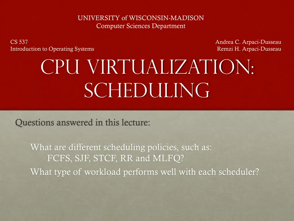
UNIVERSITY of WISCONSIN-MADISON Computer Sciences Department CS 537 Introduction to Operating Systems Andrea C. Arpaci-Dusseau Remzi H. Arpaci-Dusseau CPU Virtualization: Scheduling Questions answered in this lecture: What are different scheduling policies, such as: FCFS, SJF, STCF, RR and MLFQ? What type of workload performs well with each scheduler?

Announcements Reading: Today cover Chapters 7-9 Project 1: Sorting and System Calls Sorting : Warm-up with using C Finish Part A this week Competition: Free text book or t-shirt to fastest (average) sort in each discussion section Handin directories not yet available Goal is for everyone to learn material Do not copy code from others!

CPU Virtualization: Two Components Dispatcher (Previous lecture) Low-level mechanism Performs context-switch Switch from user mode to kernel mode Save execution state (registers) of old process in PCB Insert PCB in ready queue Load state of next process from PCB to registers Switch from kernel to user mode Jump to instruction in new user process Scheduler (Today) Policy to determine which process gets CPU when

Review: State Transitions Descheduled Running Ready Scheduled I/O: initiate I/O: done Blocked How to transition? ( mechanism ) When to transition? ( policy )

Vocabulary Workload: set of job descriptions (arrival time, run_time) Job: View as current CPU burst of a process Process alternates between CPU and I/O process moves between ready and blocked queues Scheduler: logic that decides which ready job to run Metric: measurement of scheduling quality

Scheduling Performance Metrics Minimize turnaround time Do not want to wait long for job to complete Completion_time arrival_time Minimize response time Schedule interactive jobs promptly so users see output quickly Initial_schedule_time arrival_time Minimize waiting time Do not want to spend much time in Ready queue Maximize throughput Want many jobs to complete per unit of time Maximize resource utilization Keep expensive devices busy Minimize overhead Reduce number of context switches Maximize fairness All jobs get same amount of CPU over some time interval

Workload Assumptions 1. Each job runs for the same amount of time 2. All jobs arrive at the same time 3. All jobs only use the CPU (no I/O) 4. Run-time of each job is known

Scheduling Basics Workloads: arrival_time run_time Schedulers: FIFO SJF STCF RR Metrics: turnaround_time response_time

Example: workload, scheduler, metric JOB arrival_time (s) run_time (s) A ~0 B ~0 C ~0 10 10 10 FIFO: First In, First Out - also called FCFS (first come first served) - run jobs in arrival_time order What is our turnaround?: completion_time - arrival_time

FIFO: Event Trace Time 0 0 0 0 10 10 20 20 30 Event A arrives B arrives C arrives run A complete A run B complete B run C complete C JOB arrival_time (s) run_time (s) A ~0 B ~0 C ~0 10 10 10

FIFO (Identical JOBS) A B C JOB arrival_time (s) run_time (s) A ~0 B ~0 C ~0 10 10 10 0 20 40 60 80 Gantt chart: Illustrates how jobs are scheduled over time on a CPU

FIFO (IDENTICAL JOBS) [A,B,C arrive] A B C 0 20 40 60 80 What is the average turnaround time? Def: turnaround_time = completion_time - arrival_time

FIFO (IDENTICAL Jobs) A: 10s B: 20s C: 30s 0 20 40 60 80 What is the average turnaround time? Def: turnaround_time = completion_time - arrival_time (10 + 20 + 30) / 3 = 20s

Scheduling Basics Workloads: arrival_time run_time Schedulers: FIFO SJF STCF RR Metrics: turnaround_time response_time

Workload Assumptions 1. Each job runs for the same amount of time 2. All jobs arrive at the same time 3. All jobs only use the CPU (no I/O) 4. The run-time of each job is known

Any Problematic Workloads for FIFO? Workload: ? Scheduler: FIFO Metric: turnaround is high

Example: Big First Job JOB arrival_time (s) run_time (s) A ~0 B ~0 C ~0 60 10 10 Draw Gantt chart for this workload and policy What is the average turnaround time?

Example: Big First Job JOB arrival_time (s) run_time (s) A ~0 B ~0 C ~0 60 10 10 A: 60s B: 70s C: 80s A B C 0 20 40 60 80 Average turnaround time: 70s

Convoy Effect

Passing the Tractor Problem with Previous Scheduler: FIFO: Turnaround time can suffer when short jobs must wait for long jobs New scheduler: SJF (Shortest Job First) Choose job with smallest run_time

Shortest Job First JOB arrival_time (s) run_time (s) A ~0 B ~0 C ~0 60 10 10 What is the average turnaround time with SJF?

SJF Turnaround Time A: 80s B: 10s C: 20s B C A 0 20 40 60 80 What is the average turnaround time with SJF? (80 + 10 + 20) / 3 = ~36.7s Average turnaround with FIFO: 70s For minimizing average turnaround time (with no preemption): SJF is provably optimal Moving shorter job before longer job improves turnaround time of short job more than it harms turnaround time of long job

Scheduling Basics Workloads: arrival_time run_time Schedulers: FIFO SJF STCF RR Metrics: turnaround_time response_time

Workload Assumptions 1. Each job runs for the same amount of time 2. All jobs arrive at the same time 3. All jobs only use the CPU (no I/O) 4. The run-time of each job is known

Shortest Job First (Arrival Time) JOB arrival_time (s) run_time (s) A ~0 B ~10 C ~10 60 10 10 What is the average turnaround time with SJF?

Stuck Behind a Tractor Again JOB arrival_time (s) run_time (s) A ~0 B ~10 C ~10 [B,C arrive] 60 10 10 A B C 0 20 40 60 80 What is the average turnaround time? (60 + (70 10) + (80 10)) / 3 = 63.3s

Preemptive SchedulING Prev schedulers: FIFO and SJF are non-preemptive Only schedule new job when previous job voluntarily relinquishes CPU (performs I/O or exits) New scheduler: Preemptive: Potentially schedule different job at any point by taking CPU away from running job STCF (Shortest Time-to-Completion First) Always run job that will complete the quickest

NON-PREEMPTIVE: SJF JOB arrival_time (s) run_time (s) A ~0 B ~10 C ~10 60 10 10 [B,C arrive] A B C 0 20 40 60 80 Average turnaround time: (60 + (70 10) + (80 10)) / 3 = 63.3s

PREEMPTIVE: STCF JOB arrival_time (s) run_time (s) A ~0 B ~10 C ~10 60 10 10 [B,C arrive] A: 80s B: 10s C: 20s A B C A 0 20 40 60 80 Average turnaround time with STCF? 36.6 Average turnaround time with SJF: 63.3s

Scheduling Basics Workloads: arrival_time run_time Schedulers: FIFO SJF STCF RR Metrics: turnaround_time response_time

Response Time Sometimes care about when job starts instead of when it finishes New metric: response_time = first_run_time - arrival_time

Response vs. Turnaround B s turnaround: 20s B s response: 10s A B 0 20 40 60 80 [B arrives]

Round-Robin Scheduler Prev schedulers: FIFO, SJF, and STCF can have poor response time New scheduler: RR (Round Robin) Alternate ready processes every fixed-length time-slice

FIFO vs RR ABC A B C 0 5 10 15 20 0 5 10 15 20 Avg Response Time? (0+5+10)/3 = 5 Avg Response Time? (0+1+2)/3 = 1 In what way is RR worse? Ave. turn-around time with equal job lengths is horrible Other reasons why RR could be better? If don t know run-time of each job, gives short jobs a chance to run and finish fast

Scheduling Basics Workloads: arrival_time run_time Schedulers: FIFO SJF STCF RR Metrics: turnaround_time response_time

Workload Assumptions 1. Each job runs for the same amount of time 2. All jobs arrive at the same time 3. All jobs only use the CPU (no I/O) 4. The run-time of each job is known

Not I/O Aware CPU: A A A B Disk: A A 0 20 40 60 80 Don t let Job A hold on to CPU while blocked waiting for disk

I/O Aware (Overlap) CPU: A1 B A2 B A3 B Disk: A A 0 20 40 60 80 Treat Job A as 3 separate CPU bursts When Job A completes I/O, another Job A is ready Each CPU burst is shorter than Job B, so with SCTF, Job A preempts Job B

Workload Assumptions 1. Each job runs for the same amount of time 2. All jobs arrive at the same time 3. All jobs only use the CPU (no I/O) 4. The run-time of each job is known (need smarter, fancier scheduler)

MLFQ (Multi-Level Feedback Queue) Goal: general-purpose scheduling Must support two job types with distinct goals - interactive programs care about response time - batch programs care about turnaround time Approach: multiple levels of round-robin; each level has higher priority than lower levels and preempts them

Priorities Rule 1: If priority(A) > Priority(B), A runs Rule 2: If priority(A) == Priority(B), A & B run in RR Multi-level Q3 A Q2 B How to know how to set priority? Q1 Approach 1: nice Approach 2: history feedback Q0 C D

History Use past behavior of process to predict future behavior Common technique in systems Processes alternate between I/O and CPU work Guess how CPU burst (job) will behave based on past CPU bursts (jobs) of this process

More MLFQ Rules Rule 1: If priority(A) > Priority(B), A runs Rule 2: If priority(A) == Priority(B), A & B run in RR More rules: Rule 3: Processes start at top priority Rule 4: If job uses whole slice, demote process (longer time slices at lower priorities)

One Long Job (Example) Q3 Q2 Q1 Q0 0 5 10 15 20

An Interactive Process Joins Q3 Q2 Q1 Q0 120 140 160 180 200 Interactive process never uses entire time slice, so never demoted

Problems with MLFQ? Q3 Q2 Q1 Q0 120 140 160 180 200 Problems - unforgiving + starvation - gaming the system

Prevent Starvation Q3 Q2 Q1 Q0 120 140 160 180 200 Problem: Low priority job may never get scheduled Periodically boost priority of all jobs (or all jobs that haven t been scheduled)

Prevent Gaming Q3 Q2 Q1 Q0 120 140 160 180 200 Problem: High priority job could trick scheduler and get more CPU by performing I/O right before time-slice ends Fix: Account for job s total run time at priority level (instead of just this time slice); downgrade when exceed threshold

Lottery Scheduling Goal: proportional (fair) share Approach: - give processes lottery tickets - whoever wins runs - higher priority => more tickets Amazingly simple to implement

Lottery Code int counter = 0; int winner = getrandom(0, totaltickets); node_t *current = head; while (current) { counter += current->tickets; if (counter > winner) break; current = current->next; } // current is the winner