Creating Two-Dimensional Plots Using MATLAB Graphics Functions

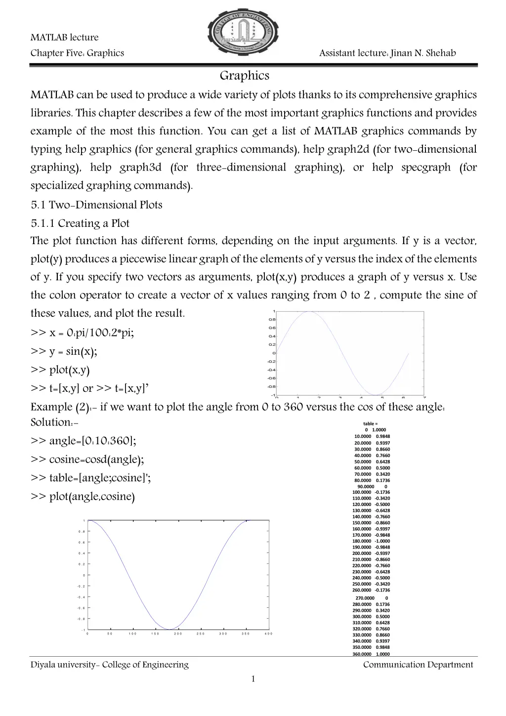
MATLAB lecture Chapter Five: Graphics Assistant lecture:Jinan N. Shehab Graphics MATLAB can be used to produce a wide variety of plots thanks to its comprehensive graphics libraries. This chapter describes a few of the most important graphics functions and provides example of the most this function. You can get a list of MATLAB graphics commands by typing help graphics (for general graphics commands), help graph2d (for two-dimensional graphing), help graph3d (for three-dimensional graphing), or help specgraph (for specialized graphing commands). 5.1 Two-Dimensional Plots 5.1.1 Creating a Plot The plot function has different forms, depending on the input arguments. If y is a vector, plot(y)produces apiecewiselineargraphof theelementsofyversustheindexoftheelements of y. If you specify two vectors as arguments, plot(x,y) produces a graph of y versus x. Use the colon operator to create a vector of x values ranging from 0 to 2 , compute the sine of these values, and plot the result. >> x = 0:pi/100:2*pi; >> y = sin(x); >> plot(x,y) >> t=[x,y] or >> t=[x,y] Example (2):- if we want to plot the angle from 0 to 360 versus the cos of these angle: Solution:- >> angle=[0:10:360]; >> cosine=cosd(angle); >> table=[angle;cosine]'; >> plot(angle,cosine) table = 0 1.0000 10.0000 20.0000 30.0000 40.0000 50.0000 60.0000 70.0000 80.0000 90.0000 0.9848 0.9397 0.8660 0.7660 0.6428 0.5000 0.3420 0.1736 0 100.0000 -0.1736 110.0000 -0.3420 120.0000 -0.5000 130.0000 -0.6428 140.0000 -0.7660 150.0000 -0.8660 160.0000 -0.9397 170.0000 -0.9848 180.0000 -1.0000 190.0000 -0.9848 200.0000 -0.9397 210.0000 -0.8660 220.0000 -0.7660 230.0000 -0.6428 240.0000 -0.5000 250.0000 -0.3420 260.0000 -0.1736 1 0 . 8 0 . 6 0 . 4 0 . 2 0 - 0 . 2 - 0 . 4 270.0000 280.0000 0.1736 290.0000 0.3420 300.0000 0.5000 310.0000 0.6428 320.0000 0.7660 330.0000 0.8660 340.0000 0.9397 350.0000 0.9848 360.0000 1.0000 Communication Department 0 - 0 . 6 - 0 . 8 - 1 0 5 0 1 0 0 1 5 0 2 0 0 2 5 0 3 0 0 3 5 0 4 0 0 Diyala university- College of Engineering 1

MATLAB lecture Chapter Five: Graphics And to label the axes and add a title( in command window or in M-file). close all clear all angle=[0:10:360]; cosine=cosd(angle); plot(angle,cosine) xlabel('angle in degree from 0 to 360') ylabel('cos angle') title('Plot of the Cosine function') Assistant lecture: Jinan N. Shehab P lo t o f th e C o s in e fu n c tio n 1 0 .8 0 .6 0 .4 0 .2 angle 0 cos -0 .2 -0 .4 -0 .6 -0 .8 -1 0 5 0 1 0 0 1 5 0 2 0 0 2 5 0 3 0 0 3 5 0 4 0 0 a n g le in d e g re e fro m 0 to 3 6 0 5.1.2 Multiple data sets in one plot Multiple (x; y) pairs arguments create multiple graphs with a single call to plot. For example, these statements plot three related functions of x: y1 = 2 cos(x), y2 = cos(x), and y3 = 0:5 cos(x), in the interval 0 ? 2?. >>x = 0:pi/100:2*pi; >> y1 = 2*cos(x); >> y2 = cos(x); >> y3 = 0.5*cos(x); >> plot(x,y1,'--',x,y2,'-',x,y3,':') >> xlabel('0 \leq x \leq 2\pi') >> ylabel('Cosine functions') >> legend('2*cos(x)','cos(x)','0.5*cos(x)') Note: the legend command provides an easy way to identify the individual plots. H.W/ Complete example (2) and (1) and draw the cosine together with the angle and sine 5.1.3 Specifying line styles and colors It is possible to specify color, line styles, and markers (such as plus signs or circles) when you plot your data using the plot command: plot(x,y,'color_style_marker') color_style_marker is a string containing from one to four characters (enclosed in single quotes) constructed from a color, a line style, and a marker type. Symbol k Black Solid 2 2*c os (x) c os (x) 1.5 0.5*c os (x) 1 0.5 0 functions Cosine -0.5 -1 -1.5 -2 0 1 2 3 4 5 6 7 0 x 2 Color Symbol Line Style Symbol + Marker Plus sign Diyala university- College of Engineering Communication Department 2

MATLAB lecture Chapter Five: Graphics r c m y g b w Assistant lecture: Jinan N. Shehab o * x . s d < Red Cyan Magenta yellow Green Blue White - - : -. None Dashed Dotted Dash-dot Noline Circle Asterisk Cross Point Square Diamond Left Triangle If you specify a marker type, but not a line style, MATLAB creates the graph using only markers, but no line. For example, plot(x,y1,'*') Another example if we want add multi-figure together plot(x,y1,'--',x,y2,'-',x,y3,':') H.W/ Plot two figure together gives (sin(x1) red with dashed line and sin(x2) green with dotted and cross marker)( don t forget legend command). 5.1.4 Graphing Imaginary and Complex Data When you pass complex values as arguments to plot, MATLAB ignores the imaginary part, except when you pass a single complex argument. For this special case, the command is a shortcut for a graph of the real part versus the imaginary part. Therefore, Example: >> plot(3+3j,'o') If z is acomplex vector or matrix, it will plot as:- Plot(real(Z), imag(Z)) Example:- >>plot([0,3],[0,9],'-+') 9 8 7 6 5 4 3 2 1 0 0 0 .5 1 1 .5 2 2 .5 3 Example:- plot the function y=eix over the interval [0,2?] with increment ? Solution:->> plot([0,3],[0,9],'-+') >> x=[0:pi/10:2*pi]; >> y=exp(x*i); >> table=[x;y]' >> plot(y,'o-') >> axis equal 1 0 . 8 0 . 6 0 . 4 0 . 2 0 -0 . 2 -0 . 4 -0 . 6 -0 . 8 - 1 - 1 -0 . 5 0 0 . 5 1 Diyala university- College of Engineering Communication Department 3

MATLAB lecture Chapter Five: Graphics After running the program it will draws a 20-sided polygon with little circles at the vertices. The command axis equal, makes the individual tick mark increments on x- and y-axes the same length which makes this plot more circular in appearance. Some useful function and command which are used in plot function:- Command plot xlabel, ylabel, zlabel title Axis [xmin, xmax], axis auto, axis square ,axis equal, axis on, axis off Assistant lecture:Jinan N. Shehab Purpose draw two-dimensional graphs define axis labels define graph title To specify the axis limit , or automatic limit selection, or x &y same size, make x visible or invisible. show labels for plot lines place text at selected locations turns grid lines on or off To add new graph to existing one, to terminate the adding graph Open new figure window if there are no figure windows already on the screen Turn the grid lines on , and off legend Text, gtext( any text ) grid Hold on, hold off figure Grid on, grid off Example:- plot the functions y1=eix andy2= sin (2x) over the interval[0,2?] with increment ? ,( first y only and second x with y). Solution:- >>x=[0:pi/10:2*pi]; >> y1=exp(x*i); >> figure(1) >> plot(y1,'-+') >> y2=sin(2*x); >> figure(2) >> plot(y2,'-o') >> axis square >> axis equal Diyala university- College of Engineering 4 1 0.8 0.6 0.4 0.2 0 -0.2 -0.4 -0.6 -0.8 -1 -1 -0.2 -0.8 -0.6 -0.4 0 0.8 0.2 0.4 0.6 1 Communication Department

MATLAB lecture Chapter Five: Graphics >> figure(3) >> plot(x,y1,'-*') Warning: Imaginary parts of complex X and/or Y arguments ignored >> figure (4) >> plot(x,y2,'-x') >> grid on Assistant lecture: Jinan N. Shehab 1 0.8 6 0.6 0.4 4 0.2 2 0 0 -0.2 -2 -0.4 -0.6 -4 -0.8 -6 -1 0 1 2 3 4 5 6 7 2 4 6 8 10 12 14 16 18 20 1 0.8 0.6 0.4 0.2 0 -0.2 -0.4 -0.6 -0.8 -1 0 1 2 3 4 5 6 7 Diyala university- College of Engineering Communication Department 5

MATLAB lecture Chapter Five: Graphics 5.1.5 Multiple plots in one figure You can displaymultiple plots in differentsub regions of the same window using the subplot function as shown below:- Subplot(m,n,p) Partitionthefigurewindowintoanm-byn-matrixofsmallsubplotandselectthepthsubplot for the current plot. The plots are numbered along first the top row of the figure window, then the second row, and so on. Example:- >>x= 0:pi/10:2*pi; >> subplot(2,2,1);plot (x,sin(x),'k*:');grid;xlabel('angle'),ylabel('sin') >> subplot(2,2,2);plot (x,cos(x),'m+-');grid;xlabel('angle'),ylabel('cos') >> subplot(2,2,3);plot (x,sin(x+pi));grid;xlabel('angle'),ylabel('sin(x+pi)') >> subplot(2,2,4);plot (x,cos(x+pi));grid;xlabel('angle'),ylabel('cos(x+pi)') Assistant lecture:Jinan N. Shehab 1 1 0 . 5 0 . 5 co 0 0 si n s -0 . 5 -0 . 5 - 1 - 1 0 2 4 6 8 0 2 4 6 8 a n g le a n g le 1 1 0 . 5 0 . 5 cos(x sin(x 0 0 +pi) +pi) -0 . 5 -0 . 5 - 1 - 1 0 2 4 6 8 0 2 4 6 8 a n g le a n g le 5.1.6 Polar coordinate graph By using (polar) function we can graph any function in polar coordinate with general form: Polar(r, ) Diyala university- College of Engineering Communication Department 6

MATLAB lecture Chapter Five: Graphics Assistant lecture: Jinan N. Shehab Example:- graph in polar coordinate the curve = + ???( ) with ?over the interval [0,4?] with dividing by 100 steps? Solution:- >>th=linspace(0,4*pi,100); >> r=1+cos(th/2); >> polar(th,r) ? 90 2 120 60 1 .5 1 150 30 0 .5 180 0 210 330 240 300 270 5.1.7 Graphing numerical functions If the function f is defined as an inline function, we can graph it with the command plot(x,f(x)). Example:- plot the sine function f(x)= sin(x) with x over the interval [0,2?] with increment 0.1 Solution:- >> f=inline('sin(x)'); >> x=[0:0.1:2*pi]; >> plot(x,f(x)) H.w/ plot cosine and two function in the same graph and rewrite (collect all function) in the M-file. 5.1.8 The ezplot command The command ezplot is used primarily to graph functions that are defined symbolically. Example:- plot the function y=sin(x) Solution: >> syms x >> y=sin(x); >> ezplot(y) And to graph it on the interval [1,5] >>ezplot(y,[1,5]) Example: find interval [1,5] Solution:- if y=x3+7x2-5x+4. Then plot the function and their derivative over the Diyala university- College of Engineering Communication Department 7

MATLAB lecture Chapter Five: Graphics >>syms x >> y=x^3+7*x^2-5*x+4; >> ezplot(y,[1:5]) >> yp=diff(y); >> figure(2) >> ezplot(yp,[1:5]) 5.2 Three-Dimensional plot:- MATLAB has a variety of functions for displaying and visualizing data in 3-D. either as lines in 3-D (plot3) , or as a wire frame (mesh) and surfaces (surf) . 5.2.1 Curves in Three-Dimensional Space For plotting curves in 3-space, the basic command is plot3, and it works like plot, except that it takes three vectors instead of two, one for the x coordinates, one for the y coordinates, and one for the z coordinates.. The command: Plot3(x,y,z) Example:- write Script file graph to plot Curve r(t) = < t*cos(t), t*sin(t), t > , if you know the ? interval t=-10 to 10?with Solution:- t = -10*pi:pi/100:10*pi; x = t.*cos(t); y = t.*sin(t); plot3(x,y,t); title('Curve u(t) = < t*cos(t), t*sin(t), t >') xlabel('x');ylabel('y'); zlabel('z') grid on 5.2.2 Surfaces in Three-Dimensional Space:- There are two basic commands for plotting surfaces in 3-space: mesh and surf. There are two different ways of using each command, one for plotting surfaces in which the z coordinate is given as a function of x and y, and one for parametric surfaces in which x, y, and z are all given as functions of two other parameters. >> mesh(X,Y,Z) Assistant lecture: Jinan N. Shehab steps. C urve u(t) = < t*c os (t), t*s in(t), t > 40 20 0 z -20 -40 40 20 40 20 0 0 -20 -20 -40 -40 y x Diyala university- College of Engineering Communication Department 8

MATLAB lecture Chapter Five: Graphics Example:-plot the surface Z=x2-y2? Solution >>[X,Y] = meshgrid(-2:.1:2, -2:.1:2); >> Z = X.^2 - Y.^2; >> mesh(X, Y, Z) Assistant lecture: Jinan N. Shehab 4 2 0 -2 -4 2 1 2 1 0 0 -1 -1 -2 -2 Example:- t = 0:pi/10:2*pi; [X,Y,Z] = cylinder(4*cos(t)); subplot(2,2,1); mesh(X); title('X'); subplot(2,2,2); mesh(Y); title('Y'); subplot(2,2,3); mesh(Z); title('Z'); subplot(2,2,4); mesh(X,Y,Z); title('X,Y,Z'); A surfaceplotis similarto ameshplotexceptthe rectangularfaces ofthesurfacearecolored. Example:-plot the surface Z=x2-y2? >> [X,Y] = meshgrid(-2:.1:2, -2:.1:2); >> Z = X.^2 - Y.^2; >> surf(X, Y, Z) % repeat this example for command surf 4 2 0 - 2 - 4 2 1 2 1 0 0 Example:- If r denotes the distance to the z axis, then the equation r2+ z2 = 1, or r= ,so x = ?, = ? ?, plot this surface. Solution:- [theta, Z] = meshgrid((0:0.1:2)*pi, (-1:0.1:1)); X = sqrt(1 - Z.^2).*cos(theta); >> Y = sqrt(1 - Z.^2).*sin(theta); surf(X, Y, Z); axis square figure(2) mesh(X,Y,Z); axis square -2 of the sphere becomes - 1 - 1 - 2 Diyala university- College of Engineering Communication Department 9