CS.121 Lecture 23 Probability Review
Lecture 23 covers a review of basic probability concepts including sample space, events, random variables, expectation, and concentration/tail bounds. The session focuses on probabilistic experiments with tossing coins and explores key principles in probability theory.

Download Presentation

Please find below an Image/Link to download the presentation.
The content on the website is provided AS IS for your information and personal use only. It may not be sold, licensed, or shared on other websites without obtaining consent from the author.If you encounter any issues during the download, it is possible that the publisher has removed the file from their server.
You are allowed to download the files provided on this website for personal or commercial use, subject to the condition that they are used lawfully. All files are the property of their respective owners.
The content on the website is provided AS IS for your information and personal use only. It may not be sold, licensed, or shared on other websites without obtaining consent from the author.
E N D
Presentation Transcript
CS 121: Lecture 23 Probability Review Madhu Sudan https://madhu.seas.Harvard.edu/courses/Fall2020 Book: https://introtcs.org { The whole staff (faster response): CS 121 Piazza How to contact us Only the course heads (slower): cs121.fall2020.course.heads@gmail.com
Announcements: Advanced section: Roei Tell (De)Randomization 2nd feedback survey Homework 6 out today. Due 12/3/2020 Section 11 week starts
Where we are: Part I: Circuits: Finite computation, quantitative study Part II: Automata: Infinite restricted computation, quantitative study Part III: Turing Machines: Infinite computation, qualitative study Part IV: Efficient Computation: Infinite computation, quantitative study Part V: Randomized computation: Extending studies to non-classical algorithms
Review of course so far Circuits: Compute every finite function but no infinite function Measure of complexity: SIZE. ALL? SIZE ? Finite Automata: Compute some infinite functions (all Regular functions) Do not compute many (easy) functions (e.g. EQ ?,? = 1 ? = ?) Turing Machines: Compute everything computable (definition/thesis) HALT is not computable: Efficient Computation: P Polytime computable Boolean functions our notion of efficiently computable NP Efficiently verifiable Boolean functions. Our wishlist NP-complete: Hardest problems in NP: 3SAT, ISET, MaxCut, EU3SAT, Subset Sum Counting 2? ? 2? ? ; ? SIZE ? Pumping/Pigeonhole Diagonalization, Reductions Polytime Reductions
Last Module: Challenges to STCT Strong Turing-Church Thesis: Everything physically computable in polynomial time can be computable in polynomial time on Turing Machine. Challenges: Randomized algorithms: Already being computed by our computers: Weather simulation, Market prediction, Quantum algorithms: Status: Randomized: May not add power? Quantum: May add power? Still can be studied with same tools. New classes: BPP,BQP: B bounded error; P Probabilistic, Q - Quantum
Today: Review of Basic Probability Sample space Events Union/intersection/negation AND/OR/NOT of events Random variables Expectation Concentration / tail bounds
Throughout this lecture Probabilistic experiment: tossing ? independent unbiased coins. Equivalently: Choose ? {0,1}?
Events Fix sample space to be ? {0,1}? An event is a set ? {0,1}?. ? 2? Probability that ? happens is Pr ? = Example: If ? {0,1}3 , Pr ?0= 1 =4 8=1 2
Q: Let ? = 3, ? = ?0= 1 ,? = ?0+ ?1+ ?2 2 ,? = {?0+ ?1+ ?2= 1 ??? 2} . What are (i) Pr[?], (ii) Pr[?], (iii) Pr[? ?], (iv) Pr[? ?] (v) Pr[? ?] ? 0 1 0 0 1 1 1 0 1 0 1 0 0 1 000 001 010 011 100 101 110 111
Q: Let ? = 3, ? = ?0= 1 ,? = ?0+ ?1+ ?2 2 ,? = {?0+ ?1+ ?2= 1 ??? 2} . What are (i) Pr[?], (ii) Pr[?], (iii) Pr[? ?], (iv) Pr[? ?] (v) Pr[? ?] ? ? ? ? ? ?=? ? ?=? ? ?=? ? ? 0 1 ? ? 0 0 1 1 1 0 1 0 1 0 0 1 000 001 010 011 100 101 110 111
Q: Let ? = 3, ? = ?0= 1 ,? = ?0+ ?1+ ?2 2 ,? = {?1+ ?2+ ?3= 1 ??? 2} . What are (i) Pr[?], (ii) Pr[?], (iii) Pr[? ?], (iv) Pr[? ?] (v) Pr[? ?] ? ? ? ? ? ?=? ? ?=? ? ?=? ? ? 0 1 ? ? Compare Pr ? ? vs Pr ? Pr[?] Pr[? ?] vs Pr ? Pr[?] 0 0 1 1 1 0 1 0 1 0 0 1 000 001 010 011 100 101 110 111
Operations on events Pr ? ?? ? ?????? = Pr[ ? ?] Pr ? ??? ? ????? = Pr[ ? ?] Pr ? ????? ? ????? = Pr ? = Pr {0,1}? ? = 1 Pr[?] Q: Prove the union bound: Pr ? ? Pr ? + Pr[?] Example: Pr ? = 4/25,Pr ? = 6/25, Pr ? ? = 9/25
Independence Pr ? ? = Pr ? Conditioning is the soul of statistics Informal: Two events ?,? are independent if knowing ?happened doesn t give any information on whether ? happened. Formal: Two events ?,? are independent if Pr ? ? = Pr ? Pr[?] Q: Which pairs are independent? (i) (ii) (iii)
More than 2 events Informal: Two events ?,? are independent if knowing whether ? happened doesn t give any information on whether ? happened. Formal: Three events ?,?,? are independent if every pair ?,? , ?,? and ?,? is independent and Pr ? ? ? = Pr ? Pr[?]Pr[?] (i) (ii)
Random variables Assign a number to every outcome of the coins. Formally r.v. is ?:{0,1}? Example: ? ? = ?0+ ?1+ ?2 ? ??[? = ?] 0 1/8 0 1 1 2 1 2 2 3 1 3/8 2 3/8 3 1/8
Expectation Average value of ? : ? ? = ? {0,1}? 2 ??(?) = ? ? Pr[? = ?] Example: ? ? = ?0+ ?1+ ?2 ? ??[? = ?] 0 1/8 1 3/8 2 3/8 0 1 1 2 1 2 2 3 3 1/8 0 1 8+ 1 3 8+ 2 3 8+ 3 1 8=12 Q: What is ?[?]? 8= 1.5
Linearity of expectation Lemma: ? ? + ? = ? ? + ?[?] Corollary: ? ?0+ ?1+ ?2 = ? ?0+ ? ?1+ ? ?2 = 1.5 Proof: ? ? + ? = 2 ? (? ? + ? ? ) = 2 ? ? ? + 2 ? ?(?) = ? ? + ?[?] ? ? ?
Independent random variables Def: ?,? are independent if {? = ?} and {? = ?} are independent ?,? Def: ?0, ,?? 1, independent if ?0= ?0, ,{?? 1= ?? 1} ind. ?0 ?? 1 i.e. ?, ,?? 1 ? [?] Pr ??= ?? = Pr[??= ??] ? ? ? ? Q: Let ? {0,1}?. Let ?0= ?0,?1= ?1, ,?? 1= ?? 1 Let ?0= ?1= = ?? 1= ?0 Are ?0, ,?? 1 independent? Are ?0, ,?? 1 independent?
Independence and concentration Q: Let ? {0,1}?. Let ?0= ?0,?1= ?1, ,?? 1= ?? 1 Let ?0= ?1= = ?? 1= ?0 Let ? = ?0+ + ?? 1 , ? = ?0+ + ?? 1 Compute ?[?], compute ?[?] For ? = 100, estimate Pr[? 0.4?,0.6? ] , Pr[? 0.4?,0.6? ]
Sums of independent random variables Pr[? 0.4,0.6 ?]= 37.5% ? = 5 https://www.stat.berkeley.edu/~stark/Java/Html/BinHist.htm
Sums of independent random variables Pr[? 0.4,0.6 ?]= 34.4% ? = 10 https://www.stat.berkeley.edu/~stark/Java/Html/BinHist.htm
Sums of independent random variables Pr[? 0.4,0.6 ?]= 26.3% ? = 20 https://www.stat.berkeley.edu/~stark/Java/Html/BinHist.htm
Sums of independent random variables Pr[? 0.4,0.6 ?]= 11.9% ? = 50 https://www.stat.berkeley.edu/~stark/Java/Html/BinHist.htm
Sums of independent random variables Pr[? 0.4,0.6 ?]= ? = 100 3.6% https://www.stat.berkeley.edu/~stark/Java/Html/BinHist.htm
Sums of independent random variables Pr[? 0.4,0.6 ?]= ? = 200 0.4% https://www.stat.berkeley.edu/~stark/Java/Html/BinHist.htm
Sums of independent random variables Pr[? 0.4,0.6 ?]= 0.01% ? = 400 https://www.stat.berkeley.edu/~stark/Java/Html/BinHist.htm
Concentration bounds ? sum of ? independent random variables Normal/Gaussian/bell curve : Pr ? 0.99,1.01 ? ? < exp( ? ?) Otherwise: weaker bounds Independent & identically distributed In concentrated r.v. s, expectation, median, mode, etc.. same Chernoff Bound: Let ?0, ,?? 1 i.i.d. r.v. s with ?? [0,1]. Then if ? = ?0+ + ?? 1 and ? = ? ? for every ? > 0, Pr ? ?? > ?? < 2 exp( 2?2 ?)
Concentration bounds ? sum of ? independent random variables Normal/Gaussian/bell curve : Pr ? 0.99,1.01 ? ? < exp( ? ?) Otherwise: weaker bounds Independent & identically distributed In concentrated r.v. s, expectation, median, mode, etc.. same Chernoff Bound: Let ?0, ,?? 1 i.i.d. r.v. s with ?? [0,1]. Then if ? = ?0+ + ?? 1 and ? = ? ? for every ? > 0, 1 ?2 Pr ? ?? > ?? < 2 exp( 2?2 ?) < exp ?2 ? if ? >
Simplest Bound: Markovs Inequality Q: Suppose that the average age in a neighborhood is 20. Prove that at most 1/4 of the residents are 80 or older. A: Suppose otherwise: 80 Contribute enough to make avg>20 Avg >1 4 80 = 20 0 >1 4 Thm (Markov s Inequality): Let ? be non-negative r.v. and ? = ?[?]. Then for every ? > 1, Pr ? ?? 1/? Proof: Same as question above
Variance & Chebychev If ? is r.v. with ? = ?[?] then ??? ? = ? ? ?2= ? ?2 ? ?2 ? ? = ???(?) Chebychev s Inequality: For every r.v. ? 1 ?2 Pr ? ? ?????????? ???? ? (Proof: Markov on ? = ? ?2 ) Compare with ? = ?? i.i.d or other r.v. s well approx. by Normal where Pr ? ? ?????????? ???? ? exp( ?2)
Next Lectures Randomized Algorithms Some examples Randomized Complexity Classes BPTIME ? ? , BPP Properties of randomized computation (Reducing error )