CUSUM Control Chart Comparison: Rule 2 vs. n out of n+k Points
The study compares the sensitivity of CUSUM Control Chart with Rule 2 using n out of n+k points as a new user rule option, exploring the effectiveness in detecting shifts and minimizing false positives. By evaluating different scenarios and probabilities, the research suggests implementing user-configurable rules to enhance the Control Chart Builder platform for more accurate process monitoring.

Download Presentation

Please find below an Image/Link to download the presentation.
The content on the website is provided AS IS for your information and personal use only. It may not be sold, licensed, or shared on other websites without obtaining consent from the author.If you encounter any issues during the download, it is possible that the publisher has removed the file from their server.
You are allowed to download the files provided on this website for personal or commercial use, subject to the condition that they are used lawfully. All files are the property of their respective owners.
The content on the website is provided AS IS for your information and personal use only. It may not be sold, licensed, or shared on other websites without obtaining consent from the author.
E N D
Presentation Transcript
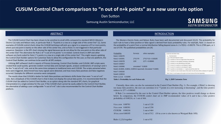
CUSUM Control Chart comparison to n out of n+k points as a new user rule option Dan Sutton Samsung Austin Semiconductor, LLC ABSTRACT INTRODUCTION The CUSUM Control Chart has been shown to be sensitive to small shifts compared to standard WECO (Western Electric Co) rules and Nelson rules, in particular Rule 2: 9 points in a row on a single side of the center line [1]. Some examples of CUSUM control charts show the CUSUM technique will pick up a signal in a sequence of 9 or more points, where just one point is barely on the other side of the center line, and so Rule 2 is not triggered in that particular sequence. Question: is the SPC chart missing the signal because we do not allow for the one point on the other side of the center line? The alternative for Rule 2 of n out of n+k points is re-visited. Control charts in JMP and other software are hard-coded for Rule 2 n points in a row on a single side of the center line . This might require updating the Control Chart Builder options for Customize Tests to allow this configuration for the user, so that one platform, the Control Chart Builder, can continue to be used for all SPC analysis. Utilizing JMP software s built in reports of Process Screening, Control Chart Builder, and CUSUM, JMP scripts were created that could quickly generate random normal data and example signals, analyze combinations of varying k and n for the n out of n+k rule, and at the same time compare to traditional tests and CUSUM. The scripts extracted when tests were triggered, determined how many signals were detected, and how many false positives and false negatives occurred. Examples for different scenarios were compared. The results show that CUSUM is better for both false positives and detects shifts faster than even n out of n+k rules. But a drawback of the CUSUM chart is that it does not display the actual data points. It is recommended that the CUSUM chart be added to Control Chart Builder, as an option along side the standard SPC charts, for graphical interpretation in a single window for the user. If the CUSUM chart cannot be easily added to the Control Chart Builder, the alternative of adding a user configurable n out of n+k rule is also recommended for the Control Chart Builder platform. The Western Electric Rules and Nelson Rules have been well documented and discussed [2],[3]. The probability for each rule to have a false positive or false signal is derived from basic probability rules. For example, Rule 1 is based on the probability of a point from a normal distribution falling beyond zones A: 2 x P(D1) = 0.00270. This is 2700 ppm, or 1 out of 370. The published probabilities are [4]: Probability Rule1: 0.00270 Rule2: 0.00391 Rule3: 0.00278 Rule4: 0.00457 Rule5: 0.00306 Rule6: (0.0045, 0.0053, 0.00553 reported). Simulated ~0.0045 Rule7: 0.00326 Rule8: 0.00010 Rules 1,2,5,6 0.01090 Table 1: Probability for each Nelson rule formula other examples 2*0.5^9 2/6! 2*0.5^10 = 0.00195 2/7! = 0.00040 simulated ~ 0.0020 Fig. 1. JMPCustomize Tests Currently, these rules can also be customized in the Control Chart Builder (Fig. 1). For example, if Rule3 is showing too many false positives, the user can customize it to 7 points in a row increasing or decreasing , and the false positive reduces to 2/7! = 0.00040. If Rule 2 is customized by the user in the Control Chart Builder options, the false positives would change as shown below. In comparison, the CUSUM control chart set to JMP recommended values of h and k has a false positive probability of 0.00216, or 1 out of 464. 8 in a row 0.00781 9 in a row 0.00391 CUSUM 10 in a row0.00195 1 out of 128 1 out of 256 1 out of 464 1 out of 512 0.00216 (10 in a row is also known as Westgard Rule 10X). Rules 1,2,5,6 together 1 out of 92
CUSUM Control Chart comparison to n out of n+k points as a new user rule option Dan Sutton Samsung Austin Semiconductor, LLC RESULTS RESULTS (continued) RESULTS (continued) Example from Engine Temperature Sensor.jmp: To see if a modified rule could be used instead of CUSUM, consider Rule 2, but allowing for one or more points to be on the other side of the center line, or n out of n+k points. False positives might go up, so need to maintain about the same false positive rate. CUSUM has a false positive rate of 1 out of 465.44 or 2.15 out of 1000, and Rule2 has a false positive rate of 1 out of 256 or 3.91 out of 1000 (added as reference lines in Fig. 2). The probabilities per 1000 runs would be: For the CUSUM chart at default settings, the shift is not detected until point 39, and the start of the shift is back calculated to point 27. For an I-MR chart, using same target and control limits, none of the WECO rules catch the trend. Figure 4: CUSUM chart Figure 5: I-MR chart (with All Rules) Comparing up to the 39thdata point, the same shift could have been detected by at least 9 out of 10, up to 13 out of 14. So can the user balance between false positives and false negatives by selecting the appropriate n out of n+k rule? Table 2: False Positive Rates for various rules Fig. 2: Graph of False Positives/1000 for varying n and k To match the false positive rate of Rule 2, proposed rules are shown in Table 3. (Note that in SAS software, for the SHEWHART procedure, one of the options is TEST2RUN (Fig. 3), which can customize the Rule 2 test in SAS software for a similar n out of n+k points rule). n k 12 out of 13 12 1 14 out of 16 14 2 16 out of 19 16 3 18 out of 22 18 4 Table 3: comparable n out of n+k rules to Rule 2 Fig. 3: Example options for TEST2RUN in SAS software Figure 6: I-MR chart but showing last 14 points.
CUSUM Control Chart comparison to n out of n+k points as a new user rule option Dan Sutton Samsung Austin Semiconductor, LLC RESULTS (continued) RESULTS (continued) RESULTS (continued) In addition to the ARL, it is also interesting to note the actual distribution of each. For small shifts of multiples of sigma, with a process following a normal distribution, we can actually see long run lengths with no signals, due to the signal continuing to be hidden by the background noise. Rule2 12 out of 13 ARL (Average Run Length): Another way to compare the different SPC rules is using the ARL (Average Run Length) to find a signal. For various shifts of 0, 0.25, 0.5, 0.75, 1 multiples of sigma, the average run length to pick up a signal can be compared. Using a JMP script, the ARL for various alternate rules were simulated (Table 4, Fig. 7). For a simulated shift, the point that the shift was detected was recorded. Note that the CUSUM ARL is much lower than comparable rules. CUSUM Table 4: ARL s for various rules and varying multiples of sigma Figure 7: Average Run Length to detect various shifts of multiple sigma. Figure 8: Distribution of Average Run Lengths for 1000 simulated examples to detect a signal for various shifts of multiple sigma.
CUSUM Control Chart comparison to n out of n+k points as a new user rule option Dan Sutton Samsung Austin Semiconductor, LLC RESULTS (continued) RESULTS (continued) RESULTS (continued) Comparing situations where CUSUM takes a long time to detect a 0.5*sigma shift, we can sometimes see another rule will pick up the signal sooner. In the example below, the CUSUM chart picked up the signal at point 154 (Fig. 9). Rule 2 picked the signal up at point 152, and continued to warn at subsequent points. But there were opportunities to pick up the signal even earlier with 10 out of 11 or 9 out of 10 signals, as well as traditional Rule 1 and Rule 5 (Fig. 11). Why are we concerned with picking up the small shift sooner? The problem is that anyone else looking at the data as just the mean of the data, might see that there is a shift of 0.05 in a particular time span (depending on binning and how much of the previous data at the 100 target is included in the calculation of the mean). (Fig. 10). The question would be why was this not detected sooner by the SPC chart? Similarly, based on ARL, there should be more cases where CUSUM picks up the signal before Rule2 or 12 out of 13. In Figure 12 below, for another example of simulated data, Rule 6 may have picked up the signal, but might be dismissed for not being persistent enough. In Figure 13 below, the CUSUM detects the shift in the mean, and also continues to warn when the shift is detected (note: the CUSUM summaries only shows when the shift was detected. The JMP user will have to add the rules to flag above and below the limits, unless there is an update to the Save Summaries). simulated data simulated data Figure 12: Simulated data with 0.5*sigma shift. Rule 6 may have detected, but not persistent signal simulated data Figure 9: Example CUSUM chart that took a long time to detect a 0.5* sigma shift. Figure 10: Underlying mean at 100.5 simulated data Figure 13: CUSUM detecting the signal and being persistent on the alarm 9 out of 10 9 out of 10 Request for CUSUM > Save Summaries that an additional column be added that shows persistent signals (as highlighted in yellow). Otherwise, JMP user has to create their own column based on LCL and UCL. Figure 11: One of the simulated examples showing Rules 1, 5, 10 out of 11, and 9 out of 10 might have detected the signal. Note that Rule 2 also triggered at points 152, 153, 154.
CUSUM Control Chart comparison to n out of n+k points as a new user rule option Dan Sutton Samsung Austin Semiconductor, LLC RESULTS (continued) RESULTS (continued) RESULTS (continued) Detection of Small Signals of Length 3 to 9 points: simulated data Now let us assume that we need to pick up a smaller signal. One example would be adding a small shift of 3 points or more, up to 9 points, of various multiples of sigma. In this scenario, we might have an intermittent assignable cause, such as a sticking valve or other temporary perturbation of the normal process. Side by side comparisons were made of the Rules 1, 2, 5, 6 compared to CUSUM and to the Rule 12of13. In a control chart of 10000 data points, 100 signals were added, and the number detected was tabulated For example, if a 7 point signal of 0.5*sigma was introduced periodically, not every signal might be detected. In Figure 14 we see an example where 2 signals are not detected by Rules 1, 2, 5, 6, but one signal is. The user may still fail to see the underlying problem. For the same example, CUSUM detects the middle shift (Figure 15), but also illustrates picking up a false signal prior to it. Finally for this example, the middle shift was also detected by 12 out of 13 rule (Figure 16). simulated data Figure 15: Same data as in Figure 14. CUSUM detects the middle signal, but also has one false positive simulated data Figure 14: Simulated data with mean=100, sigma=0.1, but 3 signals of 7 points shifted by 0.5*sigma or 0.05. Figure 16: Same data as in Figure 14. Rule 12 of 13 detects the middle signal same as CUSUM
CUSUM Control Chart comparison to n out of n+k points as a new user rule option Dan Sutton Samsung Austin Semiconductor, LLC RESULTS (continued) RESULTS (continued) RESULTS (continued) Detection of Small Signals of Length 3 to 9 points: Side by side comparisons were made of using Rules 1, 2, 5, 6 together, compared to CUSUM, and compared to the Rule 12of13. In a control chart of 10000 data points, 100 signals were added, and the number detected was tabulated, over a replication of 100 simulations. The percentage of signals detected are shown below in Table 5 and Figure 17. The use of all 4 rules 1,2,5,6 can pick up more of these signals from the underlying noise than CUSUM. For longer durations of the signal, alternate rules such as 12 of 13 can pick up this signal. Rules 1,2,5,6 CUSUM Figure 17: Percentage of signals detected for varying size signals for Rule1,2,5,6, CUSUM, and Rule1_out_of_13 Rule 12 of 13 Table 5: Same data as in Figure 14. CUSUM detects the middle signal, but also has one false positive
CUSUM Control Chart comparison to n out of n+k points as a new user rule option Dan Sutton Samsung Austin Semiconductor, LLC RECOMMENDATION RECOMMENDATION (continued) RECOMMENDATION (continued) Rules 1,2,5,6, CUSUM, and modified rules such as 12 of 13, are all just tools for SPC detection of signals. The proposal is to allow the CUSUM to be added to Control Chart Builder as an option, similar to the 3-Way Chart button, so that the user can compare the standard data points and SPC chart with the CUSUM trends side by side (Fig. 18). Additional proposal is to allow JMP users to add their own custom rules (Fig 19): n Test description Label 12 n out of n + k (k = 1) points in a row on a single side of the center line 9 or user can specify 12of13 simulated data 9 Example of proposed combined chart with the CUSUM option in same window, and with a user- configured Rule 9 added Figure 19: Example of additional customization option to the Control Chart Builder platform CONCLUSIONS The ability of the SPC chart to pick up signals, without too many false signals, has been explored for the traditional Western Electric/Nelson Rules, the CUSUM method, and n out of n+k rules. For continuous improvement, it is recommended to add to the Control Chart Builder the option to include CUSUM and one or more specialized n out of n+k rules. This will allow JMP users to have a one stop platform for SPC analysis. Figure 18: Traditional I-MR chart with CUSUM below. Dynamic linking allows same points to be seen in all charts
CUSUM Control Chart comparison to n out of n+k points as a new user rule option Dan Sutton Samsung Austin Semiconductor, LLC REFERENCES [1] A. Zangi, How to detect small shifts in Control Charts , JMPer Cable, https://community.jmp.com/t5/JMPer-Cable/How-to-detect-small-shifts-in-Control-Charts/ba-p/49452 (2018). [2] 1. Walker, E., Philpot, J.W. and Clement, J. 1991. False signal rates for the Shewhart control chart with supplementary runs tests, Journal of Quality Technology 23, 247-252. [3] Champ, C.W. and Woodall, W. 1987. Exact results for Shewhart control charts with supplementary runs rules, Technometrics 29, 393-399. [4] Griffiths, D., Bunder, M. W., Gulati, C. M. & Onizawa, T. (2010). The probability of an out of control signal from Nelson''s supplementary zig-zag test. Journal of Statistical Theory and Practice, 4 (4), 609-615. [5] T. Mauldin, Using ARL (Average Run Length) to determine the performance of a control chart , JMPer Cable, https://community.jmp.com/t5/JMPer-Cable/Using-ARL-Average-Run-Length-to-determine-the-performance-of-a/ba-p/61895 (2018).