Data Transformation and Regression Analysis

This content discusses the linearization of seemingly nonlinear relationships through data transformation in regression analysis. It covers various types of relationships such as exponential growth or decay, allometric relationships, and sigmoid relationships. The growth curve of E. coli is examined to estimate parameters like initial density and instantaneous growth rate. R functions are utilized for data analysis and plotting. Additionally, linear regression is employed to find parameters in the allometric law governing the body weight of wild elephants based on inter-leg distance.

• Data transformation
• Regression analysis
• Exponential growth
• Allometric relationships
• Sigmoid relationships

eastburn_a Follow

Uploaded on Apr 13, 2025 | 0 Views

Download Presentation

Please find below an Image/Link to download the presentation.

The content on the website is provided AS IS for your information and personal use only. It may not be sold, licensed, or shared on other websites without obtaining consent from the author.If you encounter any issues during the download, it is possible that the publisher has removed the file from their server.

You are allowed to download the files provided on this website for personal or commercial use, subject to the condition that they are used lawfully. All files are the property of their respective owners.

The content on the website is provided AS IS for your information and personal use only. It may not be sold, licensed, or shared on other websites without obtaining consent from the author.

Presentation Transcript

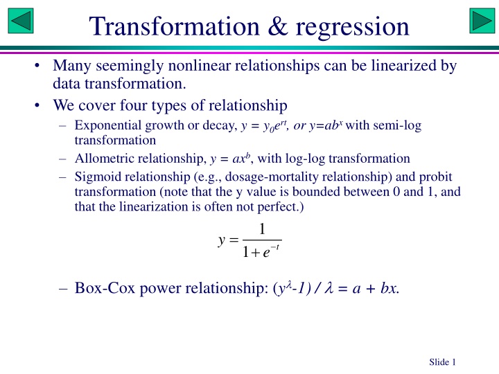
1. Transformation & regression Many seemingly nonlinear relationships can be linearized by data transformation. We cover four types of relationship Exponential growth or decay, y = y0ert, or y=abx with semi-log transformation Allometric relationship, y = axb, with log-log transformation Sigmoid relationship (e.g., dosage-mortality relationship) and probit transformation (note that the y value is bounded between 0 and 1, and that the linearization is often not perfect.) 1 = y e + t 1 Box-Cox power relationship: (y -1) / = a + bx. Slide 1

2. Growth curve of E. coli A researcher wishes to estimate the growth curve of E. coli. He put a very small number of E. coli cells into a large flask with rich growth medium, and take samples every half an hour to estimate the density (n/L). 14 data points over 7 hours were obtained. What is the instantaneous rate of growth (r). What is the initial density (N0)? As the flask is very large, he assumed that the growth should be exponential, i.e., y = a ebt (Which parameter correspond to r and which to N0?) lny = lna + bt T 0.5 1 1.5 2 2.5 3 3.5 4 4.5 5 5.5 6 6.5 7 Density 20 39 80 161 317 635 1284 2569 5082 10220 20673 40591 81374 163963 Xuhua Xia Slide 3

3. R functions Save the data in the previous slide to EcoliGrowth.txt ("clipboard" may be platform-specific) md<-read.table("EcoliGrowth.txt",header=T) attach(md) plot(T,Density) lnD <- log(Density) fit<-lm(lnD~T) # Alternatively, fit<-lm(log(Density)~T) summary(fit) anova(fit) plot(lnD~T) abline(fit) Run, and ask students to replace a and b in the equation y = a ebt by estimated numbers. What is the initial density and the instantaneous growth rate? PredY<-exp(fitted(fit)) plot(Density~T) lines(PredY~T) Does the output represent confidence limits of Density for T = 1.3? nd<-data.frame(T=1.3); predict(fit,nd,interval="confidence"); predict(fit,nd,interval="prediction"); ci95<-predict(fit,md,interval="confidence") ci95Scaled<-exp(ci95) plot(Density~T) lines(ci95Scaled[,1]~T,col="red") lines(ci95Scaled [,2]~T,col="blue") lines(ci95Scaled [,3]~T,col="blue") matplot(T, ci95Scaled, lty = c(1,2,2), type = "l", col=c("black","red","red"), ylab = "Density",xlab="T") points(Density~T)

4. Body weight of wild elephant L 0.31 1.657 0.43 2.500 0.52 4.680 0.59 7.075 0.70 10.070 0.83 11.988 0.89 14.836 1.12 18.318 1.13 23.496 1.19 27.897 1.25 36.796 1.41 44.611 1.50 51.183 1.10 ? 0.93 ? W A researcher wishes to estimate the body weight of wild elephants. He measured the body weight of 13 captured elephants of different sizes as well as a number of predictor variables, such as leg length (L), trunk length, etc. Through stepwise regression, he found that the inter-leg distance (shown in figiure) is the best predictor of body weight. He measured L approximately by placing a ruler on the path of elements and then take pictures He learned from his former biology professor that the allometric law governing the body weight (W) and the length of a body part (L) states that W = aLb Use linear regression to find parameters a and b.

5. R functions md<-read.table("ElephantWt.txt",header=T) attach(md) plot(W~L) lnL <- log(L) lnW <- log(W) fit<-lm(lnW~lnL) summary(fit) anova(fit) plot(lnW~lnL) abline(fit) Run, and ask students to replace a and b in the equation W = aLb by estimated numbers. PredW<-exp(fitted(fit)) plot(W~L) lines(PredW~L) nd<-data.frame(lnL=log(c(1.10,0.93))) predict(fit,nd,interval="confidence") ci95<-predict(fit,md,interval="confidence") ci95Scaled<-exp(ci95) plot(W~L) lines(ci95Scaled[,1] ~L,col="red") lines(ci95Scaled [,2] ~L,col="blue") lines(ci95Scaled [,3] ~L,col="blue") matplot(L, ci95Scaled, lty = c(1,2,2), type = "l", col=c("black","red","red"), ylab = "W",xlab="L") points(W~L) Xuhua Xia Slide 6

6. 95% Confidence interval plot 50 40 30 W 20 10 0 0.4 0.6 0.8 1.0 1.2 1.4 L Xuhua Xia Slide 7

7. DNA and protein gel electrophoresis How to estimate the molecular mass of a protein? A ladder: proteins with known molecular mass Deriving a calibration curve relating molecular mass (M) to migration distance (D): D = F(M) Measure D and obtain M The calibration curve is obtained by fitting a regression model Xuhua Xia Slide 8

8. Assignment 1: Protein mass The equation on the right appears to describe the relationship between D and M quite well. The data set is for a standard ladder with known Mass. Migration distance (D) is measured from the gel. Use data transformation and linear regression to obtain 1) parameters a and b, 2) a 95% confidence plot, and 3) Mass and 95% confidence limits for the two points with known D but unknown Mass. bM = D ae Mass 5 10 20 30 40 50 60 70 80 ? ? D 14.5 12.6 9.4 7.1 5.3 3.9 3.05 2.3 1.75 3.5 5.6 Xuhua Xia Slide 9

9. Assignment 2: Area and Radius Estimate area (A) by counting squares and partial squares within each circle, and radius (r) by the number of squares (and partial squares) from center to circumference. Use data transformation and linear regression to fit the relationship of A = arb to find a and b (Report the data, the fitted equation and confidence interval of area given r = 5). Xuhua Xia

10. Box-Cox power transformation x 1 4 9 17 25 33 41 49 57 65 73 81 89 97 105 113 121 129 137 y 1.1882 1.2625 1.3506 1.4348 1.4897 1.5287 1.5602 1.5857 1.6105 1.6305 1.6497 1.6654 1.6816 1.6953 1.7094 1.7214 1.7335 1.7439 1.7554 Used when we do not know the functional relationship but wish to obtain a good description and prediction. The Box-Cox power transformation aims to find a so that the transformed y is linearly related to x. ?? 1 ? = ? + ?? Criteria: 1. the best is one that will yields the highest R2 between (y -1)/ and x. 2. the best is one that will yields the largest likelihood. 3. the best is one that will minimize RSS. Likelihood function: 1. conventional for normally distributed residuals 2. ??? = ? 2ln(???? + 3. ??? = ? 2??(???? ? 1 ? ? 2 ??? (????? ??? ?? ?? 2012,?.435) 2) + ? 1 ??? (Box-Cox, 1964) Slide 11

11. Maximize R md<-read.table("PowerTransform.txt",header=T) attach(md) plot(y~x) myF<-function(lambda) abs(cor(x,(y^lambda-1)/lambda)) sol<-optimize(myF,interval=c(1,20),maximum=T); lambda<-sol$maximum newY<-(y^lambda-1)/lambda plot(newY~x) fit<-lm(newY~x) CI95<-predict(fit,md,interval="confidence") CI95Scaled<-(CI95*lambda+1)^(1/lambda) plot(y~x) lines(CI95Scaled[,1]~x,col="red") lines(CI95Scaled[,2]~x,col="black") lines(CI95Scaled[,3]~x,col="blue") The transformation originally proposed by Box and Cox (1964) also includes a scaling factor, i.e., the transformed variable is ?? 1 the transformed y will be similar. ??? 1. With this scaling factor, the standard deviation between the original y and

12. LS criterion md<-read.clipboard(header=T) attach(md) plot(y~x) myF<-function(lambda,x,y) { lnY<-log(y) if(lambda==0) { nuY<-lnY } else { nuY<-(y^lambda-1)/lambda } meanX<-mean(x); n<-length(x);DF<-n-3 numer<-(x-meanX)*nuY; denom<-(x-meanX)^2 b<-sum(numer)/sum(denom) res<- nuY-b*x; var.res<-var(res) # get lnL return(-DF/2*log(var.res)+(lambda-1)*(DF/n)*sum(lnY) ) } sol<-optimize(myF,interval=c(1,20),maximum=T,x=x,y=y) lambda<-sol$maximum newY<-(y^lambda-1)/lambda plot(newY~x); fit<-lm(newY~x) CI95<-predict(fit,md,interval="confidence") CI95Scaled<-(CI95*lambda+1)^(1/lambda) plot(y~x) lines(CI95Scaled[,1]~x,col="red"); lines(CI95Scaled[,2]~x,col="black") lines(CI95Scaled[,3]~x,col="blue") ??? = ? ? 1 ? ? 2 2ln(???? + ???

13. Confidence interval of A general method of attaching confidence interval with likelihood method: 2 ??? = 2(???best ???????) For DF = 1, 2(0.95,1) = 3.84. If 2 ??? > 3.84 or ??? > 3.84/2, then ???? is too small or too large. In our case, best = 10.00883 corresponding to ???best = 109.9772. If ???? = 9.907 or ???? = 10.111, then 2 ??? > 3.84, i.e., 9.907 is too small and 10.111 too large for ?. However, for ???? = 9.908 or ???? = 10.110, then 2 ??? < 3.84, so confidence interval for ? is (9.908, 10.110). 110 105 L 100 The code below takes this approach to find the confidence limits for ? 95 9.6 9.8 10.0 10.2 10.4 lamb lamb <- seq(from=9.5,to=10.5,by=0.001);lambL<-length(lamb) lnL<-rep(0,lambL) for(i in 1:length(lamb)) lnL[i]<-(myF(lamb[i],x,y)) lamb.Peak<-lamb[lnL>(max(lnL)-qchisq(0.95,1)/2)]; peak_lnL<-length(lamb.Peak) LL<-lamb.Peak[1];UL<-lamb.Peak[peak_lnL];LL;UL; plot(lnL~lamb) abline(h=max(L)-qchisq(0.95,1)/2,col="red") abline(v=c(LL,UL),col="blue")

14. boxcox function #There is a boxcox function in library (MASS) library(MASS) res<-boxcox(y~x,seq(from=0,to=20,by=0.01)) lambda<-res$x[which.max(res$y)] newY<-(y^lambda-1)/lambda plot(newY,x) fit<-lm(newY~x) CI95<-predict(fit,md,interval="confidence") CI95Scaled<-(CI95*lambda+1)^(1/lambda) plot(y~x) lines(CI95Scaled[,1]~x,col="red") lines(CI95Scaled[,2]~x,col="black") lines(CI95Scaled[,3]~x,col="blue") Xuhua Xia Slide 15

15. Box-Cox and polynomial 1 ?= ?? 1 ? ? + ?? = ? + ?? is equivalent to ? = 1 + ?? + ??? 1 ? , where ? = 1 + ??,and ? = ?? If = 1/2 then ? = ?0+ ?1? + ?2?2 If = 1/3 then ? = ?0+ ?1? + ?2?2+ ?3?3 If = 1/4 then ? = ?0+ ?1? + ?2?2+ ?3?3+ ?4?4 Just as polynomial regression is used for description when true functional relationship is unknown, so is Box-Cox transformation. Xuhua Xia Slide 16

16. Toxicity study: pesticide Dosage Mortality 27 35 38 44 45 46 49 50 52 53 54 56 57 58 59 60 61 62 63 64 66 68 69 100 0.9 6.42 11.71 27.45 29.96 34.3 45.71 49.86 57.68 62.92 67.14 74.12 76.77 79.01 83.53 83.96 87.95 88.74 91.13 92.64 95.49 97 97.15 90 80 70 60 Mortality (%) 50 40 30 20 10 0 25 30 35 40 45 50 55 60 65 70 Dosage What transformation to use? Data also used in a lecture for generalized linear models Xuhua Xia

17. Probit and logit transformation Probit transformation Probit has two names/definitions, both associated with standard normal distribution: the inverse cumulative distribution function (CDF) quantile function CDF is denoted by (z), which is a continuous, monotone increasing sigmoid function in the range of (0,1), e.g., (z) = p (-1.96) = 0.025 = 1 - (1.96) The probit function gives the 'inverse' computation, formally denoted -1(p), i.e., probit(p) = -1(p) probit(0.025) = -1.96 = -probit(0.975) [probit(p)] = p, and probit[ (z)] = z. Logit transformation: ln[p/(1-p)] The two transformations are applicable in similar situnations. Which one to use is largely arbitrary. 0.4 0.3 0.2 p 0.1 0.0 -3 -2 -1 0 1 2 3 z 1 0.9 0.8 0.7 0.6 CDF 0.5 0.4 0.3 0.2 0.1 0 -2.5 -1.5 -0.5 0.5 1.5 z Xuhua Xia Slide 18

18. R functions md<-read.table("Pesticide.txt",header=T) attach(md) plot(Dosage,Mortality) Why divide Percent by 100? NuProbit<-qnorm(Mortality/100) fit<-lm(NuProbit~Dosage) summary(fit) anova(fit) plot(NuProbit~Dosage) abline(fit) Run and explain Assignment: Re-do the analysis with logit transformation. PredM<-100*pnorm(fitted(fit)) plot(Mortality~Dosage) lines(PredM~Dosage) nd<-data.frame(Dosage=31) pred31<-predict(fit,nd,interval="confidence") pred31<-100*pnorm(pred31) ci95<-predict(fit,md,interval="confidence") ci95Scaled<-100*pnorm(ci95) plot(Mortality~Dosage) lines(ci95Scaled[,1]~Dosage,col="red") lines(ci95Scaled[,2]~Dosage,col="blue") lines(ci95Scaled[,3]~Dosage,col="blue") Xuhua Xia Slide 19