Decays in the MSSM with Quark Flavor Violation & Higgs Boson Studies

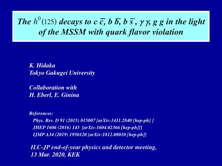
0 The decays to c c , , b b , b s , g g g g, g g in the light of the MSSM with quark flavor violation (125 ) h K. Hidaka Tokyo Gakugei University Collaboration with H. Eberl, E. Ginina References: Phys. Rev. D 91 (2015) 015007 [arXiv:1411.2840 [hep-ph] ] JHEP 1606 (2016) 143 [arXiv:1604.02366 [hep-ph]]] IJMP A34 (2019) 1950120 [arXiv:1812.08010 [hep-ph]] ILC-JP end-of-year physics and detector meeting, 13 Mar. 2020, KEK

Contents 1. Introduction 2. MSSM with QFV 3. Constraints on the MSSM 4. Parameter scan for h0 c c , b b , b s in the MSSM 5. h0 c c , b b , b s in the MSSM 6. h0 g g g g, , g g in the MSSM 7. Conclusion

~u 1. Introduction 2 , 1 What is the SM-like Higgs boson discovered at LHC? It can be the SM Higgs boson. It can be a Higgs boson of New Physics. This is one of the most important issues in the present particle physics field! 0 Here we study a possibility that it is the lightest Higgs boson of the h Minimal Supersymmetric Standard Model (MSSM), focusing on the decays h0(125) c c , b b , b s , , g g g g, , g g.

2. MSSM with QFV The basic parameters of the MSSM with QFV: tan , mA, M1, M2, M3, , , M2Q, , M2U, , M2D, , TU , TD ( (at Q = 1 TeVscale ) ) ( , , = = , , , , = = u, c, t or d, s, b) tan mA : CP odd Higgs boson mass (pole mass) ratio of VEV of the two Higgs doublets <H0 2>/<H01> M1,M2,M3 : U(1), SU(2),SU(3) gaugino masses higgsino mass parameter M2Q, left squark soft mass matrix M2U right up-type squark soft mass matrix M2D right down-type squark soft mass matrix TU trilinear coupling matrix of up-type squark and Higgs boson TD trilinear coupling matrix of down-type squark and Higgs boson

Key parameters in this study are: * QFV parameters: M M Q23 , M M U23 , M M D23 , T TU23 , T TU32, T TD23 , T TD32 * QFC parameter: T TU33, T TD33 M M Q23= (c L t Lmixing parameter) M M U23= (c R t Rmixing parameter) M M D23= (s R b Rmixing parameter) T TU23= (c R t Lmixing parameter) T TU32= (c L t Rmixing parameter) T TU33= (t L t Rmixing parameter) T TD23= (s R b Lmixing parameter) T TD32= (s L b Rmixing parameter) T TD33= (b L b Rmixing parameter)

3. Constraints on the MSSM We respect the following experimental and theoretical constraints: (1) The recent LHC limits on the masses of squarks, sleptons, gluino, charginos and neutralinos. (2) The constraint on (mA / H+ , tan ) from recent MSSM Higgs boson search at LHC. (3) The constraints on the QFV parameters from the B meson data. + + + g - B(B ) B(Bu ) B(b s ) M etc. s Bs (4) The constraints from the observed Higgs boson mass at LHC (allowing for theoretical uncertainty): 121.6 GeV < m_h0< 128.6 GeV. (5) Theoretical constraints from the vacuum stability conditions for the trilinear couplings TUaband TDab . (6) The experimental limit on SUSY contributions to the electroweak r r parameter r r(SUSY) < 0.0012.

4. Parameter scan for h0 c c , b b , b s in the MSSM - We compute the decay widths G G (h0 c c ), ), G G (h0 b b ), and G G (h0 b s ) ) at full 1-loop level in the MSSM with QFV. ), - Parameter points are generated by using random numbers in the following ranges (in units of GeV or GeV^2): 1 TeV < MSUSY < 5 TeV 10 < tan < 60 2500 < M_3 < 5000 100 < M_2 < 2500 100 < M_1 < 2500 (without assuming the GUT relation for M_1, M_2, M_3) 100 < mu < 2500 800 < m_A(pole) < 6000;

MQ2_11 = 4500^2 (fixed) 2500^2 < MQ2_22 < 4000^2 2500^2 < MQ2_33 < 4000^2 |MQ2_23| < 1000.^2 <=== QFV param. MU2_11 = 4500^2 (fixed) 1000.^2 < MU2_22 < 4000.^2 600.^2 < MU2_33 < 3000.^2 |MU2_23| < 1500.^2 <=== QFV param. MD2_11 = 4500^2 (fixed) 2500.^2 < MD2_22 < 4000.^2 1000.^2 < MD2_33 < 3000.^2 |MD2_23| < 2000.^2 ML2_11 = 1500^2 (fixed) ML2_22 = 1500^2 (fixed) ML2_33 = 1500^2 (fixed) ML2_23 = 0. (fixed)

ME2_11 = 1500^2 (fixed) ME2_22 = 1500^2 (fixed) ME2_33 = 1500^2 (fixed) ME2_23 = 0. (fixed) |TU_23| < 4000 <=== QFV param |TU_32| < 4000 <=== QFV param |TU_33| < 5000 <=== QFC param |TD_23| < 2000 |TD_32| < 2000 |TD_33| < 3000 TE_23 = 0. (fixed) TE_32 = 0. (fixed) |TE_33| < 500 <=== QFV param <=== QFV param <=== QFC param - In the parameter scan, all of the relevant experimental and theoretical constraints are imposed. - 101000 parameter points are generated and 2993 points survive the constraints.

5. h0 c c , b b , b s in the MSSM - We compute the decay widths G G (h0 c c ), ), G G (h0 b b ), ), and G G (h0 b s ) ) at full 1-loop level in the DRbar renormalization scheme in the MSSM with QFV. - Main 1-loop correction to h0 c c : gluino - su loops [ su = (t - c mixture)] - Main 1-loop corrections to h0 b b & b s : gluino sd loops [ sd = ( b - s mixture)] chargino - su loops [ su = (t - c mixture)] - The width G G (h0 c c ) ) can be measured very precisely at ILC, but it is very difficult to measure it at LHC.

~ ~ ~ ~ In large & R c t t L t mixing scenario; ~ / / L R L R ~ c + c t ~ / ~u / R L R L h0 H20 2 , 1 ~ 2 , 1 ~ ~ + u c t 0 0 2 h H ~ g ~ / / R L R L ~u 2 , 1 ~ ~ + c c t ~ / / R L R L , ~ t L ~ t ~ t ~ c ~ t ~ c In our scenario, trilinear couplings ( couplings) = (TU TU , TU ) are large! ~ u , 2 0 2 0 H H 0 2 H R R L L R ~ 0 2 , 1 u h couplings are large! 2 , 1 Gluino loop contributions can be large! Deviation of G G (h0 c c ) from SM width can be large!

Main one-loop contributions with SUSY particles

In large sR/L- bR/L & bL- bRmixing scenario; b h0 - s H10+ c H20 d 1,2 h0 d 1,2 s R/L+ b R/L g d 1,2 b / s In our scenario, trilinear couplings (TD TD , TD ) = (s R- b L- H10 , s L- b R- H10 , b L- b R- H10couplings) are large! d 1,2 - d 1,2- h0couplings are large! Gluino loop contributions can be large! Deviation of G G (h0 b b /s ) from SM width can be large!

In large cR/L- tR/L & tL- tRmixing scenario; b h0 H20 u 1,2 u 1,2 c R/L+ t R/L h0 c c c c ~ W + H u 1,2 b / s ~ ~ t ~ t ~ c ~ t ~ c , t L 0 2 0 H H 0 2 In our scenario, trilinear couplings ( couplings) = (TU TU , TU ) are large! ~ u , 2 H R R L L R ~ 0 2 , 1 u h couplings are large! 2 , 1 Chargino loop contributions can be large! Deviation of G G (h0 b b /s ) from SM width can be large!

5.1 Deviation of the width from the SM prediction - The deviation of the width from the SM prediction: _ _ _ DEV(h0-> X X) = G G(h0-> X X)MSSM/ G G (h0-> X X)SM- 1 X = c, b

Scatter plot in DEV(h0-> c c) - DEV(h0-> b b) plane Expected 1 sigma error at ILC250 + HL-LHC Expected 1 sigma error at ILC250 + HL-LHC 0.2 DEV(h0-> b b ) 0.1 DEV(b) x x SM SM 0.0 -0.1 -0.2 Expected 1 sigma error at ILC250/500 + HL-LHC Expected 1 sigma error at ILC250/500 + HL-LHC -0.8 -0.6 -0.4 -0.2 0.0 0.2 0.4 0.6 DEV(h0-> c c ) DEV(c) - DEV(h0-> c c ) and DEV(h0-> b b ) can be very large simultaneously!: DEV(h0-> c c ) can be as large as ~ DEV(h0-> b b ) can be as large as ~ 60%. 20%. - ILC can observe such large deviations from SM at high significance (arXiv:1908.11299)!: DEV(h0-> c c ) = (3.60%, 2.40%, 1.58%) at (ILC250, ILC500, ILC1000) DEV(h0-> b b ) = (1.98%, 1.16%, 0.94%) at (ILC250, ILC500, ILC1000)

Scatter plot in DEV(h0-> c c) - DEV(h0-> b b) plane 2.0 CMS (1 sigma error) CMS (1 sigma error) 1.5 ATLAS (1 sigma error) ATLAS (1 sigma error) 1.0 DEV(h0-> b b ) DEV(b) 0.5 CMS (central value) CMS (central value) ATLAS (central value) ATLAS (central value) SM SM x x 0.0 MSSM MSSM ATLAS (1 sigma error) ATLAS (1 sigma error) -0.5 CMS (1 sigma error) CMS (1 sigma error) -1.0 -0.8 -0.6 -0.4 -0.2 0.0 0.2 0.4 0.6 DEV(c) DEV(h0-> c c ) - Recent LHC data: DEV(h0-> b b ) = 0.12 +0.92/-0.62 = [-0.50, 1.04] (ATLA S) (ATLAS-CONF-2019-005) DEV(h0-> b b ) = 0.37 +1.52/-1.06 = [-0.69, 1.89] (CMS) (arXiv:1809.10733) - Both SM and MSSM are consistent with the recent ATLAS/CMS data! The errors of the recent ATLAS/CMS data are too large!

5.2 Deviation of width ratio from the SM prediction - The deviation of the width ratio from the SM prediction: DEV(b/c) = [G G (b) / G G (c)]MSSM/ [G G (b) / G G (c)]SM - 1 _ G G (X) = G G (h0-> X X)

Scatter plot in TU32 DEV(b/c) plane 2.0 1.5 1.0 DEV(b/c) DEV(b/c) 0.5 SM 0.0 -0.5 -4000 -2000 0 2000 4000 TU32 (GeV) c L t Rmixing parameter T_U32 (GeV) -There is a strong correlation between TU32 DEV(b/c)! - DEV(b/c) can be as large as ~ +200% for large TU32!

5.3 BR(h0 b s / s b) BR(h0-> b s / s b ) 0 (SM) BR(h0-> b s / s b ) can be as large as ~ 0.17% (MSSM with QFV)! ILC(250+500+1000) sensitivity could be ~ 0.1% (at 4 s s significance)! (See also Heinemeyer et al., PR D93 (2016) 095021 [arXiv:1511.04342]. )

Scatter plot in TD23- BR(h0-> b s / s b) plane 2.0x10-3 ILC(250+500+1000) sensitivity at 4 s s significance BR(h^0 -> b sb) + BR(h^0 -> bb s) 1.5 BR(h0-> b s / s b ) 0.1% 1.0 0.5 0.0 -2000 -1000 0 1000 2000 TD23 (GeV) s R b Lmixing parameter T_D23 (GeV) -There is a strong correlation between TD23- BR(h0-> b s / s b )! - BR(h0-> b s / s b ) can be as large as 0.17% for large TD23 ! - ILC(250 + 500 + 1000) sensitivity could be ~ 0.1% at 4 sigma significance! (private communication with J. Tian) - LHC &HL-LHC sensitivity should not be so good due to huge QCD BG!

Scatter plot in TD32- BR(h0-> b s / s b) plane 2.0x10-3 ILC(250+500+1000) sensitivity at 4 s s significance BR(h^0 -> b sb) + BR(h^0 -> bb s) 1.5 BR(h0-> b s / s b ) 0.1% 1.0 0.5 0.0 -2000 -1000 0 1000 2000 TD32 (GeV) s L b Rmixing parameter T_D32 (GeV) - There is also a strong correlation between TD32- BR(h0-> b s / s b )! - BR(h0-> b s / s b ) can be as large as 0.17% for large TD32!

Scatter plot in BR(h0 b s / s b) - DEV(h0 b b ) plane 2.0x10-3 ILC(250+500+1000) sensitivity at 4 s s significance BR(h^0 -> b sb) + BR(h^0 -> bb s) 1.5 BR(h0 b s / s b ) 0.1% 1.0 0.5 SM x 0.0 -0.2 -0.1 0.0 DEV(b) 0.1 0.2 DEV(h0 b b ) - There is a strong correlation between DEV(h0 b b ) & BR(h0 b s / s b )! - This is due to the fact that DEV(h0 b b ) & BR(h0 b s / s b ) have a common origin of enhancement effect, i.e. large trilinear couplings TD23,32,33& TU23,32,33.

Scatter plot in BR(h0 b s / s b) - tan plane 2.0x10-3 ILC(250+500+1000) sensitivity at 4 s s significance BR(h^0 -> b sb) + BR(h^0 -> bb s) 1.5 BR(h0 b s / s b ) 0.1% 1.0 0.5 0.0 10 20 30 40 50 60 tanb tan - There is a strong correlation between BR(h0 b s / s b ) & tan ! - BR(h0-> b s / s b ) can be as large as 0.17% for tan ~ ~ 0 0!

6. h0 g g g g, , g g in the MSSM - For the h decays to photon photon and gluon gluon we compute the widths at NLO QCD level. We perform a MSSM parameter scan respecting theoretical and experimental constraints. - From the parameter scan, we find the followings: (1) DEV(h0 g g g g ) and DEV(h0 g g) can be sizable simultaneously: DEV(h0 g g g g ) can be as large as ~ + 4%, DEV(h0 g g) can be as large as ~ -15%. (2) There is a very strong correlation between DEV(h0 g g g g ) and DEV(h0 g g). This correlation is due to the fact that the stop-loop (stop-scharm mixture loop) contributions dominate the two DEV's. (3) The deviation of the width ratio G G (h0 g g g g ) / G G (h0 g g ) in the MSSM from the SM value can be as large as ~ +20%.

Scatter plot in DEV(h0 g g g g ) - DEV(h0 g g) plane DEV(h0 g g) DEV(h0 g g g g ) - DEV(h0 g g g g ) and DEV(h0 g g) can be sizable simultaneously! -There is a strong correlation between DEV(h0 g g g g ) and DEV(h0 g g)! -This correlation is due to the fact that the stop-loop (stop-scharm mixture loop) contributions dominate the two DEV s .

Scatter plot in DEV(h0 g g g g ) - DEV(h0 g g) plane DEV(h0 g g) SM DEV(h0 g g g g ) - Both SM and MSSM are consistent with the recent ATLAS/CMS data!: ATLAS: ATLAS-CONF-2018-031 (ICHEP2018) CMS: arXiv:1804.02716 (Submitted to JHEP) - The errors of the recent ATLAS/CMS data are too large!

7. Conclusion - We have studied the decays h0(125GeV) c c , b b , b s , g g g g, , g g in the MSSM with QFV. - Performing a parameter scan respecting theoretical and experimental constraints , we have found the followings: * DEV(h0-> c c ) and DEV(h0-> b b ) can be very large simultaneously! : DEV(h0-> c c ) can be as large as ~ DEV(h0-> b b ) can be as large as ~ 60%, 20%. * The deviation of the width ratio G G (h0-> b b ) / G G (h0-> c c ) from the SM value can be as large as ~ +200%. * BR(h0-> b s / s b ) can be as large as ~ 0.17%! ILC(250 + 500 + 1000) sensitivity could be ~ 0.1% at 4 sigma signal significance!

* DEV(h0-> g g g g ) and DEV(h0-> g g) can be sizable simultaneously! : DEV(h0-> g g g g ) can be as large as ~ +4%, DEV(h0-> g g) can be as large as ~ -15%. * The deviation of the width ratio G G (h0-> g g g g )/ G G (h0-> g g) from the SM value can be as large as ~ +20%. * There is a very strong correlation between DEV(h0-> g g g g ) and DEV(h0-> g g). This correlation is due to the fact that the stop-loop (stop-scharm mixture loop) contributions dominate the two DEV's. - All of these large deviations in the h0(125GeV) decays are due to large c - t mixing & large c / t involved trilinear couplings TU32, TU23, TU33and large s - b mixing & large s / b involved trilinear couplings TD32, TD23, TD33. - ILC can observe such large deviations from SM at high significance! - In case the deviation pattern shown here is really observed at ILC, then it would strongly suggest the discovery of QFV SUSY (MSSM with QFV)! - See next slide also.

- Our analysis suggests the following: PETRA/TRISTAN e- e+ collider discovered virtual Z0 effect for the first time. Later, CERN p p collider discovered the Z0boson. Similarly, ILC could discover virtual Sparticle effects for the first time in h0(125GeV) decays! Later, HE-LHC/VLHC p p colliders could discover the Sparticles!

END Thank you!

Backup Slides

Scatter plot in TU23 DEV(b/c) plane 2.0 1.5 1.0 DEV(b/c) DEV(b/c) 0.5 SM 0.0 -0.5 -4000 -2000 0 2000 4000 TU23 (GeV) c R t Lmixing parameter T_U23 (GeV) -There is almost no correlation between TU23 DEV(b/c)! - DEV(b/c) can be as large as 200%!

Scatter plot in TU33 DEV(b/c) plane 2.0 1.5 1.0 DEV(b/c) DEV(b/c) 0.5 SM 0.0 -0.5 -4000 -2000 0 2000 4000 TU33 (GeV) t R t Lmixing parameter T_U33 (GeV) -There is almost no correlation between TU33 DEV(b/c)! - DEV(b/c) can be as large as 200%!

0.3 0.4 0.2 0.2 0.1 0.0 DEV(b) DEV(c) 0.0 -0.2 -0.1 -0.4 -0.2 -0.6 -0.3 -0.8 -4000 -2000 0 2000 4000 -4000 -2000 0 2000 4000 TU32 (GeV) TU32 (GeV) 2.0 1.5 1.0 DEV(b/c) 0.5 0.0 -0.5 -4000 -2000 0 2000 4000 TU32 (GeV)

2.0x10-3 0.2 BR(h^0 -> b sb) + BR(h^0 -> bb s) 1.5 0.1 DEV(b) 0.0 1.0 -0.1 0.5 -0.2 0.0 10 20 30 40 50 60 10 20 30 40 50 60 tanb tanb 2.0x10-3 BR(h^0 -> b sb) + BR(h^0 -> bb s) 1.5 1.0 0.5 0.0 -0.2 -0.1 0.0 DEV(b) 0.1 0.2

Constraints on the MSSM parameters from K & B meson and h0data: